pacman::p_load(sf, sfdep, tidyverse, tmap)In-Class Exercise 6: Spatial Weights - sfdep method
1 Installing and Loading the R Packages
2 The Data
For the purpose of this in-class exercise, the Hunan data sets will be used. There are two data sets in this use case, they are:
Hunan, a geospatial data set in ESRI shapefile format, and
Hunan_2012, an attribute data set in csv format
2.1 Importing geospatial data
Import the data as an sf format.
hunan <- st_read(dsn="data/geospatial",
                 layer="Hunan")
Reading layer `Hunan' from data source
`C:\guga-nesh\IS415-GAA\in-class_ex\in-class_ex06\data\geospatial'
using driver `ESRI Shapefile'
Simple feature collection with 88 features and 7 fields
Geometry type: POLYGON
Dimension: XY
Bounding box: xmin: 108.7831 ymin: 24.6342 xmax: 114.2544 ymax: 30.12812
Geodetic CRS: WGS 84# geographic coordinate system is not good for distance-based metrics, but if you're going for contiguity its ok2.2 Importing attribute table
Import the data as a tibble data frame.
hunan_2012 <- read_csv("data/aspatial/Hunan_2012.csv")

hunan_2012
# A tibble: 88 × 29
County City avg_w…¹ depos…² FAI Gov_Rev Gov_Exp GDP GDPPC GIO
<chr> <chr> <dbl> <dbl> <dbl> <dbl> <dbl> <dbl> <dbl> <dbl>
1 Anhua Yiyang 30544 10967 6832. 457. 2703 13225 14567 9277.
2 Anren Chenzhou 28058 4599. 6386. 221. 1455. 4941. 12761 4189.
3 Anxiang Changde 31935 5517. 3541 244. 1780. 12482 23667 5109.
4 Baojing Hunan W… 30843 2250 1005. 193. 1379. 4088. 14563 3624.
5 Chaling Zhuzhou 31251 8241. 6508. 620. 1947 11585 20078 9158.
6 Changning Hengyang 28518 10860 7920 770. 2632. 19886 24418 37392
7 Changsha Changsha 54540 24332 33624 5350 7886. 88009 88656 51361
8 Chengbu Shaoyang 28597 2581. 1922. 161. 1192. 2570. 10132 1681.
9 Chenxi Huaihua 33580 4990 5818. 460. 1724. 7755. 17026 6644.
10 Cili Zhangji… 33099 8117. 4498. 500. 2306. 11378 18714 5843.
# … with 78 more rows, 19 more variables: Loan <dbl>, NIPCR <dbl>, Bed <dbl>,
# Emp <dbl>, EmpR <dbl>, EmpRT <dbl>, Pri_Stu <dbl>, Sec_Stu <dbl>,
# Household <dbl>, Household_R <dbl>, NOIP <dbl>, Pop_R <dbl>, RSCG <dbl>,
# Pop_T <dbl>, Agri <dbl>, Service <dbl>, Disp_Inc <dbl>, RORP <dbl>,
# ROREmp <dbl>, and abbreviated variable names ¹avg_wage, ²deposite2.3 Combining both data frames using left join
Combine the spatial and aspatial data. Since one is the tibble data frame and he other is an sf object, to retain geospatial properties, the left data frame must be sf (i.e., hunan)
# left_join() keeps all observations in x
# in this case, we did not mention the common identifier - by default uses common field
# after they have been joined, I want only columns 1-4, 7, and 15 (basically I just want the GDPPC from the hunan_2012)

hunan_GDPPC <- left_join(hunan, hunan_2012) %>%
  select(1:4, 7, 15)

hunan_GDPPC
Simple feature collection with 88 features and 6 fields
Geometry type: POLYGON
Dimension: XY
Bounding box: xmin: 108.7831 ymin: 24.6342 xmax: 114.2544 ymax: 30.12812
Geodetic CRS: WGS 84
First 10 features:
NAME_2 ID_3 NAME_3 ENGTYPE_3 County GDPPC
1 Changde 21098 Anxiang County Anxiang 23667
2 Changde 21100 Hanshou County Hanshou 20981
3 Changde 21101 Jinshi County City Jinshi 34592
4 Changde 21102 Li County Li 24473
5 Changde 21103 Linli County Linli 25554
6 Changde 21104 Shimen County Shimen 27137
7 Changsha 21109 Liuyang County City Liuyang 63118
8 Changsha 21110 Ningxiang County Ningxiang 62202
9 Changsha 21111 Wangcheng County Wangcheng 70666
10 Chenzhou 21112 Anren County Anren 12761
geometry
1 POLYGON ((112.0625 29.75523...
2 POLYGON ((112.2288 29.11684...
3 POLYGON ((111.8927 29.6013,...
4 POLYGON ((111.3731 29.94649...
5 POLYGON ((111.6324 29.76288...
6 POLYGON ((110.8825 30.11675...
7 POLYGON ((113.9905 28.5682,...
8 POLYGON ((112.7181 28.38299...
9 POLYGON ((112.7914 28.52688...
10 POLYGON ((113.1757 26.82734...2.4 Plotting Choropleth Map
tmap_mode("plot")

tm_shape(hunan_GDPPC)+
  tm_fill("GDPPC",
          style = "quantile",
          palette = "Blues",
          title = "GDPPC") +
  tm_layout(main.title = "Distribution of GDP per capita by district, Hunan Province",
            main.title.position = "center",
            main.title.size = 0.8,
            legend.height = 0.35,
            legend.width = 0.25,
            frame = TRUE) +
  tm_borders(alpha = 0.5) +
  tm_compass(type="8star", size = 1) +
  tm_scale_bar() +
  tm_grid(alpha =0.2)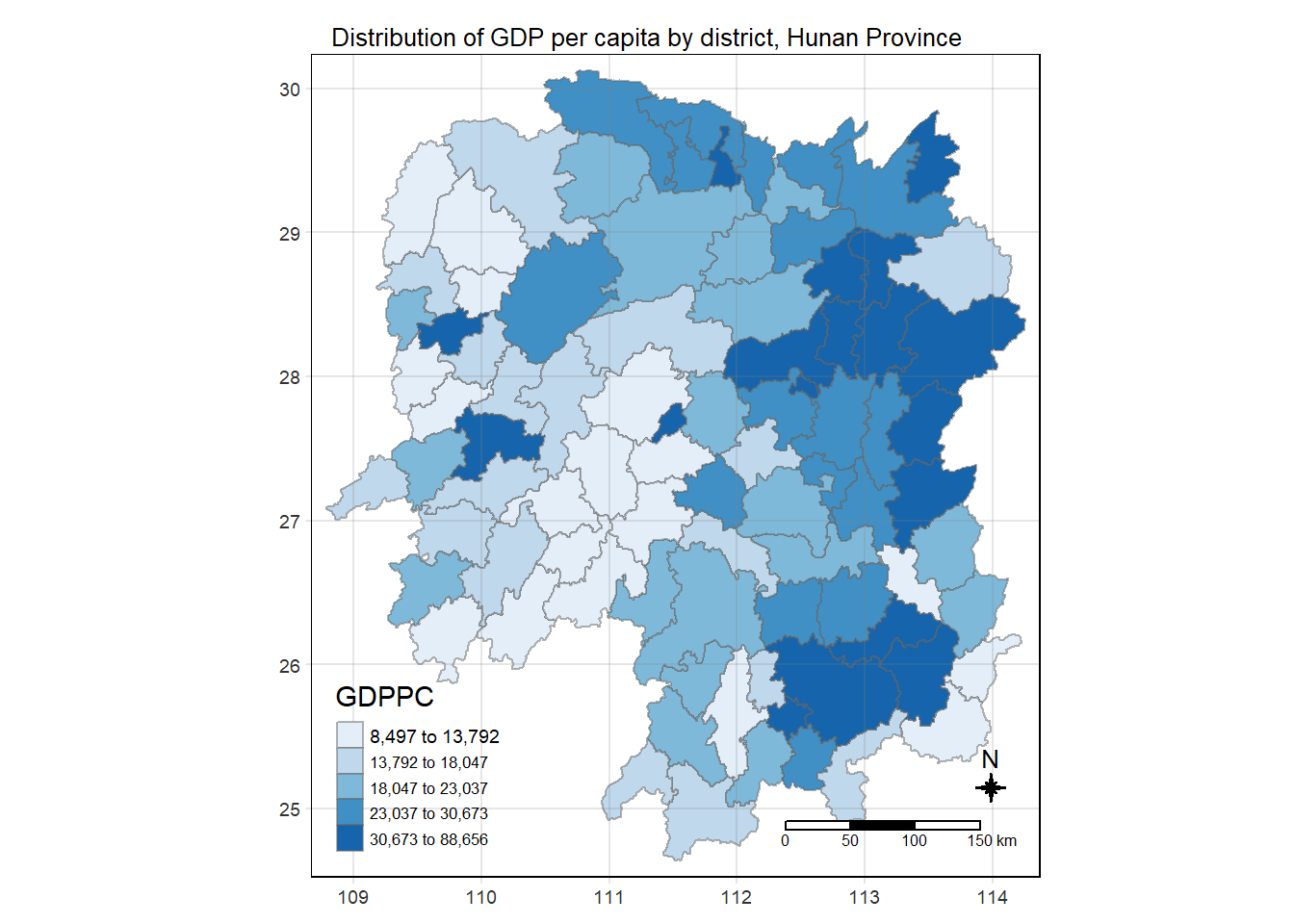
# remember tm_fill and tm_borders will give you the tm_polygon, we do it like this to have a higher level of control on the visuals

# always output the map first to see where you can place the map components like scale bar, compass, etc.

# Classification Method: if you are designing for a regional economic study then you might want to use "equal interval" classification method. It depends on the purpose of our study.
3 Deriving Contiguity Spatial Weights
There are two main types of spatial weights, they are contiguity weights and distance-based weights. In this section, we will be focusing on contiguity spatial weights using sfdep.
There are two main steps to derive contiguity spatial weights:
- identifying contiguity neighbour list using
st_contiguity()of sfdep package. - deriving the contiguity spatial weights using
st_weights()of sfdep package.
3.1 Identify contiguity neighbours: Queen’s method
Before the spatial weight matrix can be derived, the neighbours need to be identified first.
st_contiguity() is used to derive contiguity neighbour list using Queen’s method. Documentation can be found here. Some key information:
It only works for sf geometry type
POLYGONorMULTIPOLYGON.By default, it uses queen (i.e.,
spdep::poly2nb).
cn_queen <- hunan_GDPPC %>%
  mutate(nb = st_contiguity(geometry),
         .before=1)

# use dplyr::mutate() to create new field that stores st_contiguity() on the geometry field
# .before = 1 basically puts the newly created field in the first column
The code chunk below is used to print the summary of the first lag neighbour list (i.e., nb).
summary(cn_queen$nb)Neighbour list object:
Number of regions: 88
Number of nonzero links: 448
Percentage nonzero weights: 5.785124
Average number of links: 5.090909
Link number distribution:
1 2 3 4 5 6 7 8 9 11
2 2 12 16 24 14 11 4 2 1
2 least connected regions:
30 65 with 1 link
1 most connected region:
85 with 11 linksThe output above shows that there are 88 area units in Hunan province. The most connected area has 11 neighbours. There are two units with only 1 neighbour.
Let’s view the table
cn_queenSimple feature collection with 88 features and 7 fields
Geometry type: POLYGON
Dimension: XY
Bounding box: xmin: 108.7831 ymin: 24.6342 xmax: 114.2544 ymax: 30.12812
Geodetic CRS: WGS 84
First 10 features:
nb NAME_2 ID_3 NAME_3 ENGTYPE_3
1 2, 3, 4, 57, 85 Changde 21098 Anxiang County
2 1, 57, 58, 78, 85 Changde 21100 Hanshou County
3 1, 4, 5, 85 Changde 21101 Jinshi County City
4 1, 3, 5, 6 Changde 21102 Li County
5 3, 4, 6, 85 Changde 21103 Linli County
6 4, 5, 69, 75, 85 Changde 21104 Shimen County
7 67, 71, 74, 84 Changsha 21109 Liuyang County City
8 9, 46, 47, 56, 78, 80, 86 Changsha 21110 Ningxiang County
9 8, 66, 68, 78, 84, 86 Changsha 21111 Wangcheng County
10 16, 17, 19, 20, 22, 70, 72, 73 Chenzhou 21112 Anren County
County GDPPC geometry
1 Anxiang 23667 POLYGON ((112.0625 29.75523...
2 Hanshou 20981 POLYGON ((112.2288 29.11684...
3 Jinshi 34592 POLYGON ((111.8927 29.6013,...
4 Li 24473 POLYGON ((111.3731 29.94649...
5 Linli 25554 POLYGON ((111.6324 29.76288...
6 Shimen 27137 POLYGON ((110.8825 30.11675...
7 Liuyang 63118 POLYGON ((113.9905 28.5682,...
8 Ningxiang 62202 POLYGON ((112.7181 28.38299...
9 Wangcheng 70666 POLYGON ((112.7914 28.52688...
10 Anren 12761 POLYGON ((113.1757 26.82734...The above output shows that polygon 1 has 5 neighbours: 2, 3, 4, 57, and 85. We can reveal the country name of the neighbours by using the code chunk below.
cn_queen$County[c(2,3,4,57,85)][1] "Hanshou" "Jinshi" "Li" "Nan" "Taoyuan"3.2 Identify contiguity neighbours: Rook’s method
cn_rook <- hunan_GDPPC %>%
  mutate(nb = st_contiguity(geometry,
                            queen=FALSE),
         .before=1)
3.3 Identifying higher order neighbours
Sometimes we need to identify high order contiguity neighbours. “High order” refers to the number of dimensions involved in the space. For instance, “first-order” contiguity neighbours are the immediate neighbours of a given point, while the “second-order” contiguity neighbours are the neighbours of the immediate neighbours.
To accomplish the task, st_nb_lg_cumul() should be used as shown in the code chunk below.
cn2_queen <- hunan_GDPPC %>%
  mutate(nb = st_contiguity(geometry),
         nb2 = st_nb_lag_cumul(nb, 2),
         .before = 1)
Note that if the order is 2, the result contains both 1st and 2nd order neighbours as shown on the print below.
cn2_queenSimple feature collection with 88 features and 8 fields
Geometry type: POLYGON
Dimension: XY
Bounding box: xmin: 108.7831 ymin: 24.6342 xmax: 114.2544 ymax: 30.12812
Geodetic CRS: WGS 84
First 10 features:
nb
1 2, 3, 4, 57, 85
2 1, 57, 58, 78, 85
3 1, 4, 5, 85
4 1, 3, 5, 6
5 3, 4, 6, 85
6 4, 5, 69, 75, 85
7 67, 71, 74, 84
8 9, 46, 47, 56, 78, 80, 86
9 8, 66, 68, 78, 84, 86
10 16, 17, 19, 20, 22, 70, 72, 73
nb2
1 2, 3, 4, 5, 6, 32, 56, 57, 58, 64, 69, 75, 76, 78, 85
2 1, 3, 4, 5, 6, 8, 9, 32, 56, 57, 58, 64, 68, 69, 75, 76, 78, 85
3 1, 2, 4, 5, 6, 32, 56, 57, 69, 75, 78, 85
4 1, 2, 3, 5, 6, 57, 69, 75, 85
5 1, 2, 3, 4, 6, 32, 56, 57, 69, 75, 78, 85
6 1, 2, 3, 4, 5, 32, 53, 55, 56, 57, 69, 75, 78, 85
7 9, 19, 66, 67, 71, 73, 74, 76, 84, 86
8 2, 9, 19, 21, 31, 32, 34, 35, 36, 41, 45, 46, 47, 56, 58, 66, 68, 74, 78, 80, 84, 85, 86
9 2, 7, 8, 19, 21, 35, 46, 47, 56, 58, 66, 67, 68, 74, 76, 78, 80, 84, 85, 86
10 11, 14, 15, 16, 17, 18, 19, 20, 21, 22, 23, 70, 71, 72, 73, 74, 82, 83, 86
NAME_2 ID_3 NAME_3 ENGTYPE_3 County GDPPC
1 Changde 21098 Anxiang County Anxiang 23667
2 Changde 21100 Hanshou County Hanshou 20981
3 Changde 21101 Jinshi County City Jinshi 34592
4 Changde 21102 Li County Li 24473
5 Changde 21103 Linli County Linli 25554
6 Changde 21104 Shimen County Shimen 27137
7 Changsha 21109 Liuyang County City Liuyang 63118
8 Changsha 21110 Ningxiang County Ningxiang 62202
9 Changsha 21111 Wangcheng County Wangcheng 70666
10 Chenzhou 21112 Anren County Anren 12761
geometry
1 POLYGON ((112.0625 29.75523...
2 POLYGON ((112.2288 29.11684...
3 POLYGON ((111.8927 29.6013,...
4 POLYGON ((111.3731 29.94649...
5 POLYGON ((111.6324 29.76288...
6 POLYGON ((110.8825 30.11675...
7 POLYGON ((113.9905 28.5682,...
8 POLYGON ((112.7181 28.38299...
9 POLYGON ((112.7914 28.52688...
10 POLYGON ((113.1757 26.82734...3.4 Deriving contiguity weights: Queen’s method
Now, we are ready to compute the contiguity weights by using st_weights() of sfdep package.
In the code chunk below, queen method is used to derive the contiguity weights.
cw_queen <- hunan_GDPPC %>%
  mutate(nb = st_contiguity(geometry),
         wt = st_weights(nb,
                         style="W"),
         .before = 1)
Note that st_weights() provides 3 arguments:
nb: A neighbour list object created by
st_contiguity()style: Default “W” for row standardized weights (sum over all links to n). Other options include “B”, “C”, “U”, “minmax”, “S”. B is the basic binary coding, C is globally standardised (sums over all links to n), U is equal to C / number of neighbours (sum over all links to unity), while S is the variance-stabilizing coding scheme proposed by Tiefelsdorf et al. 1999, p. 167-168 (sums over all links to n).
allow_zero: if
TRUE, assigns zero as lagged value to zone without neighbours.
cw_queenSimple feature collection with 88 features and 8 fields
Geometry type: POLYGON
Dimension: XY
Bounding box: xmin: 108.7831 ymin: 24.6342 xmax: 114.2544 ymax: 30.12812
Geodetic CRS: WGS 84
First 10 features:
nb
1 2, 3, 4, 57, 85
2 1, 57, 58, 78, 85
3 1, 4, 5, 85
4 1, 3, 5, 6
5 3, 4, 6, 85
6 4, 5, 69, 75, 85
7 67, 71, 74, 84
8 9, 46, 47, 56, 78, 80, 86
9 8, 66, 68, 78, 84, 86
10 16, 17, 19, 20, 22, 70, 72, 73
wt
1 0.2, 0.2, 0.2, 0.2, 0.2
2 0.2, 0.2, 0.2, 0.2, 0.2
3 0.25, 0.25, 0.25, 0.25
4 0.25, 0.25, 0.25, 0.25
5 0.25, 0.25, 0.25, 0.25
6 0.2, 0.2, 0.2, 0.2, 0.2
7 0.25, 0.25, 0.25, 0.25
8 0.1428571, 0.1428571, 0.1428571, 0.1428571, 0.1428571, 0.1428571, 0.1428571
9 0.1666667, 0.1666667, 0.1666667, 0.1666667, 0.1666667, 0.1666667
10 0.125, 0.125, 0.125, 0.125, 0.125, 0.125, 0.125, 0.125
NAME_2 ID_3 NAME_3 ENGTYPE_3 County GDPPC
1 Changde 21098 Anxiang County Anxiang 23667
2 Changde 21100 Hanshou County Hanshou 20981
3 Changde 21101 Jinshi County City Jinshi 34592
4 Changde 21102 Li County Li 24473
5 Changde 21103 Linli County Linli 25554
6 Changde 21104 Shimen County Shimen 27137
7 Changsha 21109 Liuyang County City Liuyang 63118
8 Changsha 21110 Ningxiang County Ningxiang 62202
9 Changsha 21111 Wangcheng County Wangcheng 70666
10 Chenzhou 21112 Anren County Anren 12761
geometry
1 POLYGON ((112.0625 29.75523...
2 POLYGON ((112.2288 29.11684...
3 POLYGON ((111.8927 29.6013,...
4 POLYGON ((111.3731 29.94649...
5 POLYGON ((111.6324 29.76288...
6 POLYGON ((110.8825 30.11675...
7 POLYGON ((113.9905 28.5682,...
8 POLYGON ((112.7181 28.38299...
9 POLYGON ((112.7914 28.52688...
10 POLYGON ((113.1757 26.82734...3.5 Deriving contiguity weights: Rook’s method
# is it supposed to be hunan_GDPPC
cw_rooks <- hunan %>%
  mutate(nb = st_contiguity(geometry,
                            queen = FALSE),
         wt = st_weights(nb),
         .before = 1)
4 Deriving Distance-based Weights
There are 3 popularly used distance-based spatial weights:
fixed distance weights
adaptive distance weights
inverse distance weights (IDW)
4.1 Deriving fixed distance weights
Before we can derive the fixed distance weights, we need to determine the upper limit for distance band by using the steps below:
geo <- sf::st_geometry(hunan_GDPPC)

# st_geometry() used to get geometry from an sf object

nb <- st_knn(geo, longlat = TRUE)

# st_knn() identifies the k nearest neighbours for given point geometry. The longlat argument is to tell if point coordinates are long-lat decimal degrees (measures in km).

dists <- unlist(st_nb_dists(geo, nb))

# st_nb_dists() of sfdep is used to calculate the nearest neighbour distance. The output is a list of distances for each observation's neighbour list.

# unlist() of Base R is used to return the output as a vector so the summary statistics of the nearest neighbour distances can be derived.
Now we can derive the summary statistics of the nearest neighbour distances vector (i.e., dists) by using the code chunk below.
summary(dists) Min. 1st Qu. Median Mean 3rd Qu. Max.
21.56 29.11 36.89 37.34 43.21 65.80 From the output above we know that the maximum nearest neighbour distance is 65.80km. By using a threshold value of 66km we will ensure that each area will have at least one neighbour.
Let’s compute the fixed distance weights by using the code chunk below.
dw_fd <- hunan_GDPPC %>%
  mutate(nb = st_dist_band(geometry,
                           upper = 66),
         wt = st_weights(nb),
         .before=1)

# st_dists_band() of sfdep is used to identify neighbours based on a distance band (i.e., 66km). The output is a list of neighbours (i.e., nb).

# st_weights() is then used to calculate polygon spatial weights of the nb list.
  # The default style argument is set to "W"
  # the default allow_zero arg. is set to TRUE, assigns ZERO as lagged value to zone without neighbours.
4.2 Deriving adaptive distance weights
dw_ad <- hunan_GDPPC %>%
  mutate(nb = st_knn(geometry,
                     k=8),
         wt = st_weights(nb),
               .before = 1)

# st_knn() of sfdep is used to identify neighbours based on k (i.e., k=8 indicates the nearest eight neighbours). The output is a list of neighbours (i.e., nb)
4.3 Calculating inverse distance weights
dw_idw <- hunan_GDPPC %>%
  mutate(nb = st_contiguity(geometry),
         wts = st_inverse_distance(nb, geometry,
                                   scale = 1,
                                   alpha = 1),
         .before = 1)

# st_inverse_distance() is used to calculate inverse distance weights of neighbours on the nb list.