Code for Package Installation
pacman::p_load(olsrr, ggpubr, sf, spdep, GWmodel, tmap, tidyverse, gtsummary, onemapsgapi, rvest, stringr, httr, jsonlite, readr, gdata, matrixStats, units, ranger, SpatialML, car, Metrics, gridExtra)Conventional predictive models for housing resale prices were built using the Ordinary Least Square (OLS) method, but this approach doesn’t consider the presence of spatial autocorrelation and spatial heterogeneity in geographic data sets. The existence of spatial autocorrelation means that using OLS to estimate predictive housing resale pricing models could result in biased, inconsistent, or inefficient outcomes. For this exercise, we will be using Geographical Weighted Models (GWR) to calibrate a predictive model for housing resale prices. Please feel free to follow along.
Before I begin, I would like to mention that this exercise was done by with the help of many resources online, including some of my seniors’ works. All references have been mentioned at the end of this webpage. Please do refer to them should you require any further explanation.
For this exercise, we will be using the independent variables recommended by Professor Kam. Please view them here.
| Type | Name | Format | Source |
|---|---|---|---|
| Geospatial | MPSZ-2019 | .shp | Professor Kam Tin Seong |
| Aspatial | Resale Flat Prices | .csv | data.gov.sg |
| Geospatial | Bus Stop locations (Feb 2023) | .shp | LTA Data Mall |
| Geospatial | Parks | .shp | OneMapSG API |
| Geospatial | Hawker Centres | .shp | OneMapSG API |
| Geospatial | Supermarkets | .geojson | data.gov.sg |
| Geospatial | MRT & LRT Stations (Train Station Exit Point) | .csv | LTA Data Mall |
| Geospatial | Shopping Malls | .csv | Wikipedia |
| Geospatial | Primary Schools | .csv | data.gov.sg |
| Geospatial | Eldercare | .shp | OneMapSG API |
| Geospatial | Childcare Centres | .shp | OneMapSG API |
| Geospatial | Kindergartens | .shp | OneMapSG API |
pacman::p_load(olsrr, ggpubr, sf, spdep, GWmodel, tmap, tidyverse, gtsummary, onemapsgapi, rvest, stringr, httr, jsonlite, readr, gdata, matrixStats, units, ranger, SpatialML, car, Metrics, gridExtra)We will need to prepare the geospatial data and by the end of this section, we should have the locations of all the points-of-interest (e.g., Primary Schools, Shopping Malls, Supermarkets, etc.) in a .shp, .csv, or .geojson format. While I was able to find data for Bus Stop locations and MRT & LRT Stations, the rest were not readily available on the Internet. Here is how I collated the rest of the data…
(1) OneMapSG API
The data was extracted by calling the OpenMapSG API. Most API endpoints in OneMapSG require a token. Please register for one here if you would like to perform some of the steps shown below.
I used the get_theme() function to retrieve the location coordinates of facilities. If we only have the facility name, we can even use the /commonapi/search endpoint to retrieve coordinates of a particular facility (this was used for the Primary School data set retrieved from data.gov.sg)
(2) Webscrap data from websites using rvest library
Some facilities’ names had to be webscrapped from Wikipedia using the rvest package. The OneMapSG API /commonapi/search endpoint was then used on the names of the facilities extracted to get the longitude and latitude (this was used to collect the Mall data).
(3) Download .shp, .geojson files from LTA or data.gov.sg
The shapefiles and geojson files were directly downloaded from LTA Data Mall or data.gov.sg and read as an sf object using st_read().
Here are the codes I used to get the data for the following facilities-of-interest:
# search for themes related to "health"
health_themes = onemapsgapi::search_themes(token, "health")
# pick a suitable theme from the output above
# use get_themes() with the queryname of the theme selected
eldercare_tibble = onemapsgapi::get_theme(token, "eldercare")
# convert it into an sf object
eldercare_sf = st_as_sf(eldercare_tibble, coords=c("Lng", "Lat"), crs=4326)
# let's write it into a shapefile for recurrent use
st_write(eldercare_sf, dsn="data/geospatial", layer="eldercare", driver= "ESRI Shapefile")# search for themes related to "parks"
park_themes = onemapsgapi::search_themes(token, "parks")
# pick a suitable theme from the output above
# use get_themes() with the queryname of the theme selected
parks_tibble = onemapsgapi::get_theme(token, "nationalparks")
# convert it into an sf object
parks_sf = st_as_sf(parks_tibble, coords=c("Lng", "Lat"), crs=4326)
# let's write it into a shapefile for recurrent use
st_write(parks_sf, dsn="data/geospatial", layer="parks", driver= "ESRI Shapefile")hawker_themes = onemapsgapi::search_themes(token, "hawker")
hawker_tibble = onemapsgapi::get_theme(token, "hawkercentre")
hawker_sf = st_as_sf(hawker_tibble, coords=c("Lng", "Lat"), crs=4326)
st_write(hawker_sf, dsn="data/geospatial", layer="hawker", driver= "ESRI Shapefile")all_themes = onemapsgapi::search_themes(token)
kindergarten_tibble = onemapsgapi::get_theme(token, "kindergartens")
kindergarten_sf = st_as_sf(kindergarten_tibble, coords=c("Lng", "Lat"), crs=4326)
st_write(kindergarten_sf, dsn="data/geospatial", layer="kindergarten", driver= "ESRI Shapefile")all_themes = onemapsgapi::search_themes(token)
childcare_tibble = onemapsgapi::get_theme(token, "childcare")
childcare_sf = st_as_sf(childcare_tibble, coords=c("Lng", "Lat"), crs=4326)
st_write(childcare_sf, dsn="data/geospatial", layer="childcare", driver= "ESRI Shapefile")To get the latest shopping mall data, I had to scrape the data off of Wikipedia. There is an amazing guide by GitHub user ValaryLim that I referenced for this section. I managed to get a pretty accurate list of shopping malls in Singapore (including the smaller ones in the Heartlands).
# from the wiki page we can see that the malls are all in unordered lists
url = "https://en.wikipedia.org/wiki/List_of_shopping_malls_in_Singapore"
document <- read_html(url)
ul_li_elems <- as.list(document %>% html_elements("ul") %>% html_elements("li") %>% html_text())
# remove those that aren't malls
temp <- ul_li_elems[-c(1:46)]
temp <- temp[-c(168:170)]
temp <- temp[-c(341:360)]
# there are duplicated malls - let's remove them
temp = as.list(gsub("\\[[^][]*]", "", temp))
temp = as.list(gsub("\\([^][]*)", "", temp))
temp = as.list(toupper(temp))
temp = as.list(gsub("THE", "", temp))
temp = trim(temp)
all_malls = as.list(unique(temp))
# remove duplicates and malls that are not operational
all_malls = all_malls[-c(176, 31, 203, 204, 205, 206, 207, 208, 209, 210, 211, 212, 213, 214, 215, 216, 217, 218, 20, 193, 185, 169, 191)]
# some of the mall names are not accurate - let's change them!
all_malls[[39]] = "GR.ID"
all_malls[[95]] = "DJIT SUN MALL"
all_malls[[42]] = "SHAW HOUSE"
all_malls[[198]] = "SHAW CENTRE"
all_malls[[51]] = "TEKKA MARKET"
all_malls[[158]] = "GRANTRAL MALL @ CLEMENTI"
all_malls[[199]] = "GRANTRAL MALL @ MACPHERSON"
all_malls[[176]] = "CAPITOL BUILDING SINGAPORE"
all_malls[[117]] = "NORTHSHORE PLAZA I"
all_malls[[200]] = "NORTHSHORE PLAZA II"
# replace spaces with %20 - so we can use it in the api endpoint
all_malls = as.list(gsub(" ", "%20", all_malls))With all the mall names, let’s use the OneMapSG API to retrieve the lat and long coords.
# get lat and lng data using onemapsg api
get_lat_lng <- function(location) {
result = tryCatch({
query = str_glue("https://developers.onemap.sg/commonapi/search?searchVal={location}&returnGeom=Y&getAddrDetails=Y")
print(query)
res = GET(query)
res_data = fromJSON(rawToChar(res$content))$results[1,]
lat = res_data$LATITUDE
lng = res_data$LONGITUDE
return (c(lat, lng))
},
error = function(e) {
print(e)
return(c("INVALID LOCATION", "INVALID LOCATION"))
})
}
shopping_mall_df = data.frame()
# h = hash()
for (mall in all_malls) {
lat_long = get_lat_lng(mall)
# print(lat_long)
name = gsub("%20", " ", mall)
# h[[str_glue("{name}")]] = lat_long
row <- c(str_glue("{name}"), lat_long[[1]], lat_long[[2]])
shopping_mall_df <- rbind(shopping_mall_df, row)
}
# rename dataframe
colnames(shopping_mall_df) <- c("Mall", "Lat", "Lng")
# let's manually retrieve the lat and lng values for those that can't be retrieved using the API
shopping_mall_df$Lat[shopping_mall_df$Mall == "CITY GATE MALL"] <- "1.30231590504573"
shopping_mall_df$Lng[shopping_mall_df$Mall == "CITY GATE MALL"] <- "103.862331661034"
shopping_mall_df$Lat[shopping_mall_df$Mall == "CLARKE QUAY CENTRAL"] <- "1.2887904"
shopping_mall_df$Lng[shopping_mall_df$Mall == "CLARKE QUAY CENTRAL"] <- "103.8424709"
shopping_mall_df$Lat[shopping_mall_df$Mall == "MANDARIN GALLERY"] <- "1.3021529"
shopping_mall_df$Lng[shopping_mall_df$Mall == "MANDARIN GALLERY"] <- "103.8363372"
shopping_mall_df$Lat[shopping_mall_df$Mall == "OD MALL"] <- "1.3379938"
shopping_mall_df$Lng[shopping_mall_df$Mall == "OD MALL"] <- "103.7935013"
# some of the lat and lng retrieved are incorrect so let's manually fix them
# the correct coords were manually found on the onemapsg website
shopping_mall_df$Lat[shopping_mall_df$Mall == "ADELPHI"] <- "1.29118503658447"
shopping_mall_df$Lng[shopping_mall_df$Mall == "ADELPHI"] <- "103.851184338699"
shopping_mall_df$Lat[shopping_mall_df$Mall == "APERIA"] <- "1.3110137"
shopping_mall_df$Lng[shopping_mall_df$Mall == "APERIA"] <- "103.8639307"
shopping_mall_df$Lat[shopping_mall_df$Mall == "BEDOK MALL"] <- "1.3248556"
shopping_mall_df$Lng[shopping_mall_df$Mall == "BEDOK MALL"] <- "103.9292532"
shopping_mall_df$Lat[shopping_mall_df$Mall == "BUANGKOK SQUARE"] <- "1.3845127"
shopping_mall_df$Lng[shopping_mall_df$Mall == "BUANGKOK SQUARE"] <- "103.8816655"
shopping_mall_df$Lat[shopping_mall_df$Mall == "BUGIS JUNCTION"] <- "1.2993706"
shopping_mall_df$Lng[shopping_mall_df$Mall == "BUGIS JUNCTION"] <- "103.8554388"
shopping_mall_df$Lat[shopping_mall_df$Mall == "BUGIS+"] <- "1.2996817"
shopping_mall_df$Lng[shopping_mall_df$Mall == "BUGIS+"] <- "103.8543123"
shopping_mall_df$Lat[shopping_mall_df$Mall == "CATHAY"] <- "1.2992061"
shopping_mall_df$Lng[shopping_mall_df$Mall == "CATHAY"] <- "103.8478268"
shopping_mall_df$Lat[shopping_mall_df$Mall == "CENTREPOINT"] <- "1.3019784"
shopping_mall_df$Lng[shopping_mall_df$Mall == "CENTREPOINT"] <- "103.8397590"
shopping_mall_df$Lat[shopping_mall_df$Mall == "CHINATOWN POINT"] <- "1.2851156"
shopping_mall_df$Lng[shopping_mall_df$Mall == "CHINATOWN POINT"] <- "103.8447261"
shopping_mall_df$Lat[shopping_mall_df$Mall == "CLEMENTI MALL"] <- "1.3148962"
shopping_mall_df$Lng[shopping_mall_df$Mall == "CLEMENTI MALL"] <- "103.7644231"
shopping_mall_df$Lat[shopping_mall_df$Mall == "DUO"] <- "1.2995343"
shopping_mall_df$Lng[shopping_mall_df$Mall == "DUO"] <- "103.8584017"
shopping_mall_df$Lat[shopping_mall_df$Mall == "ELIAS MALL"] <- "1.3786093"
shopping_mall_df$Lng[shopping_mall_df$Mall == "ELIAS MALL"] <- "103.9420270"
shopping_mall_df$Lat[shopping_mall_df$Mall == "ESPLANADE MALL"] <- "1.2896478"
shopping_mall_df$Lng[shopping_mall_df$Mall == "ESPLANADE MALL"] <- "103.8562673"
shopping_mall_df$Lat[shopping_mall_df$Mall == "FORUM SHOPPING MALL"] <- "1.3060975"
shopping_mall_df$Lng[shopping_mall_df$Mall == "FORUM SHOPPING MALL"] <- "103.8286786"
shopping_mall_df$Lat[shopping_mall_df$Mall == "HDB HUB"] <- "1.3320088"
shopping_mall_df$Lng[shopping_mall_df$Mall == "HDB HUB"] <- "103.8485316"
shopping_mall_df$Lat[shopping_mall_df$Mall == "HOUGANG 1"] <- "1.3757153"
shopping_mall_df$Lng[shopping_mall_df$Mall == "HOUGANG 1"] <- "103.8794723"
shopping_mall_df$Lat[shopping_mall_df$Mall == "ION ORCHARD"] <- "1.3039797"
shopping_mall_df$Lng[shopping_mall_df$Mall == "ION ORCHARD"] <- "103.8320323"
shopping_mall_df$Lat[shopping_mall_df$Mall == "MARINA BAY SANDS"] <- "1.2834542"
shopping_mall_df$Lng[shopping_mall_df$Mall == "MARINA BAY SANDS"] <- "103.8608090"
shopping_mall_df$Lat[shopping_mall_df$Mall == "NOVENA SQUARE"] <- "1.3199675"
shopping_mall_df$Lng[shopping_mall_df$Mall == "NOVENA SQUARE"] <- "103.8438506"
shopping_mall_df$Lat[shopping_mall_df$Mall == "ORCHARD GATEWAY"] <- "1.3004433"
shopping_mall_df$Lng[shopping_mall_df$Mall == "ORCHARD GATEWAY"] <- "103.8394428"
shopping_mall_df$Lat[shopping_mall_df$Mall == "PEOPLE'S PARK COMPLEX"] <- "1.2841340"
shopping_mall_df$Lng[shopping_mall_df$Mall == "PEOPLE'S PARK COMPLEX"] <- "103.8425200"
shopping_mall_df$Lat[shopping_mall_df$Mall == "PEOPLE'S PARK CENTRE"] <- "1.2857701"
shopping_mall_df$Lng[shopping_mall_df$Mall == "PEOPLE'S PARK CENTRE"] <- "103.8439801"
shopping_mall_df$Lat[shopping_mall_df$Mall == "POIZ"] <- "1.3313212"
shopping_mall_df$Lng[shopping_mall_df$Mall == "POIZ"] <- "103.8680699"
shopping_mall_df$Lat[shopping_mall_df$Mall == "SENGKANG GRAND MALL"] <- "1.3829816"
shopping_mall_df$Lng[shopping_mall_df$Mall == "SENGKANG GRAND MALL"] <- "103.8927210"
shopping_mall_df$Lat[shopping_mall_df$Mall == "SHAW HOUSE"] <- "1.3058481"
shopping_mall_df$Lng[shopping_mall_df$Mall == "SHAW HOUSE"] <- "103.8315082"
shopping_mall_df$Lat[shopping_mall_df$Mall == "SOUTH BEACH"] <- "1.2948335"
shopping_mall_df$Lng[shopping_mall_df$Mall == "SOUTH BEACH"] <- "103.8560375"
shopping_mall_df$Lat[shopping_mall_df$Mall == "SQUARE 2"] <- "1.3207051"
shopping_mall_df$Lng[shopping_mall_df$Mall == "SQUARE 2"] <- "103.8441607"
shopping_mall_df$Lat[shopping_mall_df$Mall == "TAMPINES 1"] <- "1.3543014"
shopping_mall_df$Lng[shopping_mall_df$Mall == "TAMPINES 1"] <- "103.9450922"
shopping_mall_df$Lat[shopping_mall_df$Mall == "TANJONG PAGAR CENTRE"] <- "1.2765836"
shopping_mall_df$Lng[shopping_mall_df$Mall == "TANJONG PAGAR CENTRE"] <- "103.8459363"
shopping_mall_df$Lat[shopping_mall_df$Mall == "TEKKA MARKET"] <- "1.3061777"
shopping_mall_df$Lng[shopping_mall_df$Mall == "TEKKA MARKET"] <- "103.8506100"
# remove VELOCITY - it's in NOVENA SQUARE which is already accounted for
shopping_mall_df = shopping_mall_df %>% filter(Mall != "VELOCITY@NOVENA SQUARE")With that we have all the malls and their locational data in a data.frame. Let’s convert this into a .csv file so we can use it later on.
write.csv(shopping_mall_df, "data/geospatial/mall.csv")Using this dataset from data.gov.sg, I only used the school name to get the lat and lng data using the OneMapSG API.
get_lat_lng <- function(location) {
result = tryCatch({
query = str_glue("https://developers.onemap.sg/commonapi/search?searchVal={location}&returnGeom=Y&getAddrDetails=Y")
print(query)
res = GET(query)
res_data = fromJSON(rawToChar(res$content))$results[1,]
lat = res_data$LATITUDE
lng = res_data$LONGITUDE
return (c(lat, lng))
},
error = function(e) {
print(e)
return(c("INVALID LOCATION", "INVALID LOCATION"))
})
}# as mentioned earlier I got this dataset from data.gov.sg - I will read it, filter out all the primary schools, and extract the names
school_info <- readr::read_csv("data/geospatial/school_info.csv")
primary_schools = as.list(subset(school_info, mainlevel_code == "PRIMARY" | mainlevel_code == "MIXED LEVELS")$school_name)
# remove those that aren't primary schools
primary_schools <- primary_schools[-c(8, 44, 74, 101, 111, 134, 136, 142, 149, 157, 169)]
# use the onemapsg api to retrive lat and lng coords
primary_schools_df = data.frame()
for (school in primary_schools) {
temp = gsub(" ", "%20", school)
lat_long = get_lat_lng(temp)
row <- c(school, lat_long[[1]], lat_long[[2]])
primary_schools_df <- rbind(primary_schools_df, row)
}
# rename the dataframe columns
colnames(primary_schools_df) <- c("School", "Lat", "Lng")While we have retrieved the data, some of them are wrong. Let’s manually rectify this.
primary_schools_df$Lat[primary_schools_df$School == "JURONG PRIMARY SCHOOL
"] <- "1.348861338692006"
primary_schools_df$Lng[primary_schools_df$School == "JURONG PRIMARY SCHOOL
"] <- "103.73297053951389"
primary_schools_df$Lat[primary_schools_df$School == "KUO CHUAN PRESBYTERIAN PRIMARY SCHOOL"] <- "1.349716245801766"
primary_schools_df$Lng[primary_schools_df$School == "KUO CHUAN PRESBYTERIAN PRIMARY SCHOOL"] <- "103.8552420147255"
primary_schools_df$Lat[primary_schools_df$School == "MAYFLOWER PRIMARY SCHOOL
"] <- "1.3776322593463508"
primary_schools_df$Lng[primary_schools_df$School == "MAYFLOWER PRIMARY SCHOOL
"] <- "103.84324844673546"
primary_schools_df$Lat[primary_schools_df$School == "METHODIST GIRLS' SCHOOL(PRIMARY)"] <- "1.3331343330353658"
primary_schools_df$Lng[primary_schools_df$School == "METHODIST GIRLS' SCHOOL(PRIMARY)"] <- "103.78342078588985"
primary_schools_df$Lat[primary_schools_df$School == "PUNGGOL PRIMARY SCHOOL"] <- "1.377228287998256"
primary_schools_df$Lng[primary_schools_df$School == "PUNGGOL PRIMARY SCHOOL"] <- "103.89467211203765"
primary_schools_df$Lat[primary_schools_df$School == "ST. ANTHONY'S PRIMARY SCHOOL"] <- "1.3643281311526845"
primary_schools_df$Lng[primary_schools_df$School == "ST. ANTHONY'S PRIMARY SCHOOL"] <- "103.74890532821937"
primary_schools_df$Lat[primary_schools_df$School == "TAMPINES PRIMARY SCHOOL"] <- "1.3498992868953197"
primary_schools_df$Lng[primary_schools_df$School == "TAMPINES PRIMARY SCHOOL"] <- "103.94425668320217"
primary_schools_df$Lat[primary_schools_df$School == "TAO NAN SCHOOL"] <- "1.305174050370657"
primary_schools_df$Lng[primary_schools_df$School == "TAO NAN SCHOOL"] <- "103.91138035251849"
primary_schools_df = primary_schools_df[! (primary_schools_df$School == "JUYING PRIMARY SCHOOL"),]Let’s save this data.frame into a csv file for us to use later on
write.csv(primary_schools_df, "data/geospatial/school.csv")sg_sf <- st_read(dsn = "data/geospatial", layer = "MPSZ-2019")Reading layer `MPSZ-2019' from data source
`C:\guga-nesh\IS415-GAA\take-home_ex\take-home_ex03\data\geospatial'
using driver `ESRI Shapefile'
Simple feature collection with 332 features and 6 fields
Geometry type: MULTIPOLYGON
Dimension: XY
Bounding box: xmin: 103.6057 ymin: 1.158699 xmax: 104.0885 ymax: 1.470775
Geodetic CRS: WGS 84eldercares_sf <- st_read(dsn = "data/geospatial", layer = "eldercare")Reading layer `eldercare' from data source
`C:\guga-nesh\IS415-GAA\take-home_ex\take-home_ex03\data\geospatial'
using driver `ESRI Shapefile'
Simple feature collection with 133 features and 4 fields
Geometry type: POINT
Dimension: XY
Bounding box: xmin: 103.7119 ymin: 1.271472 xmax: 103.9561 ymax: 1.439561
Geodetic CRS: WGS 84hawkers_sf <- st_read(dsn = "data/geospatial", layer = "hawker")Reading layer `hawker' from data source
`C:\guga-nesh\IS415-GAA\take-home_ex\take-home_ex03\data\geospatial'
using driver `ESRI Shapefile'
Simple feature collection with 125 features and 18 fields
Geometry type: POINT
Dimension: XY
Bounding box: xmin: 103.6974 ymin: 1.272716 xmax: 103.9882 ymax: 1.449017
Geodetic CRS: WGS 84trains_sf <- st_read(dsn = "data/geospatial", layer = "Train_Station_Exit_Layer")Reading layer `Train_Station_Exit_Layer' from data source
`C:\guga-nesh\IS415-GAA\take-home_ex\take-home_ex03\data\geospatial'
using driver `ESRI Shapefile'
Simple feature collection with 562 features and 2 fields
Geometry type: POINT
Dimension: XY
Bounding box: xmin: 6134.086 ymin: 27499.7 xmax: 45356.36 ymax: 47865.92
Projected CRS: SVY21parks_sf <- st_read(dsn = "data/geospatial", layer = "parks")Reading layer `parks' from data source
`C:\guga-nesh\IS415-GAA\take-home_ex\take-home_ex03\data\geospatial'
using driver `ESRI Shapefile'
Simple feature collection with 421 features and 2 fields
Geometry type: POINT
Dimension: XY
Bounding box: xmin: 103.6929 ymin: 1.214491 xmax: 104.0538 ymax: 1.462094
Geodetic CRS: WGS 84malls <- read_csv("data/geospatial/mall.csv")
# for now we will be reading the data using EPSG:4326 (i.e., WGS84)
malls_sf <- st_as_sf(malls, coords = c("Lng", "Lat"), crs=4326)supermarkets_sf <- st_read("data/geospatial/supermarkets-geojson.geojson")Reading layer `supermarkets-geojson' from data source
`C:\guga-nesh\IS415-GAA\take-home_ex\take-home_ex03\data\geospatial\supermarkets-geojson.geojson'
using driver `GeoJSON'
Simple feature collection with 526 features and 2 fields
Geometry type: POINT
Dimension: XYZ
Bounding box: xmin: 103.6258 ymin: 1.24715 xmax: 104.0036 ymax: 1.461526
z_range: zmin: 0 zmax: 0
Geodetic CRS: WGS 84kindergartens_sf <- st_read(dsn = "data/geospatial", layer = "kindergarten")Reading layer `kindergarten' from data source
`C:\guga-nesh\IS415-GAA\take-home_ex\take-home_ex03\data\geospatial'
using driver `ESRI Shapefile'
Simple feature collection with 448 features and 5 fields
Geometry type: POINT
Dimension: XY
Bounding box: xmin: 103.6887 ymin: 1.247759 xmax: 103.9717 ymax: 1.455452
Geodetic CRS: WGS 84childcares_sf <- st_read(dsn = "data/geospatial", layer = "childcare")Reading layer `childcare' from data source
`C:\guga-nesh\IS415-GAA\take-home_ex\take-home_ex03\data\geospatial'
using driver `ESRI Shapefile'
Simple feature collection with 1925 features and 5 fields
Geometry type: POINT
Dimension: XY
Bounding box: xmin: 103.6878 ymin: 1.247759 xmax: 103.9897 ymax: 1.462134
Geodetic CRS: WGS 84busstops_sf <- st_read(dsn = "data/geospatial", layer = "BusStop")Reading layer `BusStop' from data source
`C:\guga-nesh\IS415-GAA\take-home_ex\take-home_ex03\data\geospatial'
using driver `ESRI Shapefile'
Simple feature collection with 5159 features and 3 fields
Geometry type: POINT
Dimension: XY
Bounding box: xmin: 3970.122 ymin: 26482.1 xmax: 48284.56 ymax: 52983.82
Projected CRS: SVY21pri_schs <- read_csv("data/geospatial/school.csv")
# for now we will be reading the data using EPSG:4326 (i.e., WGS84)
pri_schs_sf <- st_as_sf(pri_schs, coords = c("Lng", "Lat"), crs=4326)resale_tbl <- read_csv("data/aspatial/resale-flat-prices-based-on-registration-date-from-jan-2017-onwards.csv")
# filtering the data
# train set: Jan '21 - Dec '22
# test set: Jan '23 - Feb '23
# for the purposes of this study we will be looking at 3 Room Flats ONLY
three_rm_flats = resale_tbl %>% filter(flat_type == "3 ROOM")
resale_tbl <- three_rm_flats %>% filter(month >= "2021-01")
# take a look at the dataframe with glimpse()
glimpse(resale_tbl)From the previous section, we saw that the data sets are not using Singapore’s Projected Coordinate System (i.e., SVY21 - EPSG:3414). This is just one of the issues we will need to fix in this section. Here’s what we will be doing:
select()st_is_valid() and missing values using is.na()st_transform()For our geospatial data sets we only need to know the name of the facility and the geometry column. So let’s remove all the unnecessary ones using select()
# for the geospatial datasets, the facility names are all in the first col
busstops_sf <- busstops_sf %>% select(c(1))
childcares_sf <- childcares_sf %>% select(c(1))
eldercares_sf <- eldercares_sf %>% select(c(1))
hawkers_sf <- hawkers_sf %>% select(c(1))
kindergartens_sf <- kindergartens_sf %>% select(c(1))
malls_sf <- malls_sf %>% select(c(1))
parks_sf <- parks_sf %>% select(c(1))
pri_schs_sf <- pri_schs_sf %>% select(c(1))
# for this supermarket dataset, the names of the facilities were not given
supermarkets_sf <- supermarkets_sf %>% select(c(1))
# for the trains dataset, each train has multiple exits - as such, it will be wise to put the Exit point together with the name of the stations to differentiate them
trains_sf$NAME <- paste(trains_sf$stn_name, toupper(trains_sf$exit_code))
trains_sf <- trains_sf %>% select(c(4))# returns number of invalid geometries
print(length(which(st_is_valid(busstops_sf) == FALSE)))[1] 0# return rows that contain NA values
print(busstops_sf[rowSums(is.na(busstops_sf)) != 0,])Simple feature collection with 0 features and 1 field
Bounding box: xmin: NA ymin: NA xmax: NA ymax: NA
Projected CRS: SVY21
[1] BUS_STOP_N geometry
<0 rows> (or 0-length row.names)# returns number of invalid geometries
print(length(which(st_is_valid(trains_sf) == FALSE)))[1] 0# return rows that contain NA values
print(trains_sf[rowSums(is.na(trains_sf)) != 0,])Simple feature collection with 0 features and 1 field
Bounding box: xmin: NA ymin: NA xmax: NA ymax: NA
Projected CRS: SVY21
[1] NAME geometry
<0 rows> (or 0-length row.names)# returns number of invalid geometries
length(which(st_is_valid(childcares_sf) == FALSE))[1] 0# return rows that contain NA values
print(childcares_sf[rowSums(is.na(childcares_sf)) != 0,])Simple feature collection with 0 features and 1 field
Bounding box: xmin: NA ymin: NA xmax: NA ymax: NA
Geodetic CRS: WGS 84
[1] NAME geometry
<0 rows> (or 0-length row.names)# returns number of invalid geometries
length(which(st_is_valid(eldercares_sf) == FALSE))[1] 0# return rows that contain NA values
print(eldercares_sf[rowSums(is.na(eldercares_sf)) != 0,])Simple feature collection with 0 features and 1 field
Bounding box: xmin: NA ymin: NA xmax: NA ymax: NA
Geodetic CRS: WGS 84
[1] NAME geometry
<0 rows> (or 0-length row.names)# returns number of invalid geometries
length(which(st_is_valid(hawkers_sf) == FALSE))[1] 0# return rows that contain NA values
print(hawkers_sf[rowSums(is.na(hawkers_sf)) != 0,])Simple feature collection with 0 features and 1 field
Bounding box: xmin: NA ymin: NA xmax: NA ymax: NA
Geodetic CRS: WGS 84
[1] NAME geometry
<0 rows> (or 0-length row.names)# returns number of invalid geometries
length(which(st_is_valid(kindergartens_sf) == FALSE))[1] 0# return rows that contain NA values
print(kindergartens_sf[rowSums(is.na(kindergartens_sf)) != 0,])Simple feature collection with 0 features and 1 field
Bounding box: xmin: NA ymin: NA xmax: NA ymax: NA
Geodetic CRS: WGS 84
[1] NAME geometry
<0 rows> (or 0-length row.names)# returns number of invalid geometries
length(which(st_is_valid(malls_sf) == FALSE))[1] 0# return rows that contain NA values
print(malls_sf[rowSums(is.na(malls_sf)) != 0,])Simple feature collection with 0 features and 1 field
Bounding box: xmin: NA ymin: NA xmax: NA ymax: NA
Geodetic CRS: WGS 84
# A tibble: 0 × 2
# … with 2 variables: Mall <chr>, geometry <GEOMETRY [°]># returns number of invalid geometries
length(which(st_is_valid(parks_sf) == FALSE))[1] 0# return rows that contain NA values
print(parks_sf[rowSums(is.na(parks_sf)) != 0,])Simple feature collection with 0 features and 1 field
Bounding box: xmin: NA ymin: NA xmax: NA ymax: NA
Geodetic CRS: WGS 84
[1] NAME geometry
<0 rows> (or 0-length row.names)# returns number of invalid geometries
length(which(st_is_valid(pri_schs_sf) == FALSE))[1] 0# return rows that contain NA values
print(pri_schs_sf[rowSums(is.na(pri_schs_sf)) != 0,])Simple feature collection with 0 features and 1 field
Bounding box: xmin: NA ymin: NA xmax: NA ymax: NA
Geodetic CRS: WGS 84
# A tibble: 0 × 2
# … with 2 variables: School <chr>, geometry <GEOMETRY [°]># returns number of invalid geometries
length(which(st_is_valid(supermarkets_sf) == FALSE))[1] 0# return rows that contain NA values
print(supermarkets_sf[rowSums(is.na(supermarkets_sf)) != 0,])Simple feature collection with 0 features and 1 field
Bounding box: xmin: NA ymin: NA xmax: NA ymax: NA
Geodetic CRS: WGS 84
[1] Name geometry
<0 rows> (or 0-length row.names)# returns number of invalid geometries
length(which(st_is_valid(sg_sf) == FALSE))[1] 6# return rows that contain NA values
print(sg_sf[rowSums(is.na(sg_sf)) != 0,])Simple feature collection with 0 features and 6 fields
Bounding box: xmin: NA ymin: NA xmax: NA ymax: NA
Geodetic CRS: WGS 84
[1] SUBZONE_N SUBZONE_C PLN_AREA_N PLN_AREA_C REGION_N REGION_C geometry
<0 rows> (or 0-length row.names)Great news! There are no missing values. However, we can see that sg_sf has 6 invalid geometries. Let’s fix this using st_make_valid()
# returns number of invalid geometries
sg_sf <- st_make_valid(sg_sf)
length(which(st_is_valid(sg_sf) == FALSE))[1] 0It worked! Now, we can move on to transforming the Coordinate Reference Systems.
We will be using the st_transform() method to do this.
sg_sf <- st_transform(sg_sf, 3414)
# use st_crs() to check if the crs was assigned correctly
st_crs(sg_sf)Coordinate Reference System:
User input: EPSG:3414
wkt:
PROJCRS["SVY21 / Singapore TM",
BASEGEOGCRS["SVY21",
DATUM["SVY21",
ELLIPSOID["WGS 84",6378137,298.257223563,
LENGTHUNIT["metre",1]]],
PRIMEM["Greenwich",0,
ANGLEUNIT["degree",0.0174532925199433]],
ID["EPSG",4757]],
CONVERSION["Singapore Transverse Mercator",
METHOD["Transverse Mercator",
ID["EPSG",9807]],
PARAMETER["Latitude of natural origin",1.36666666666667,
ANGLEUNIT["degree",0.0174532925199433],
ID["EPSG",8801]],
PARAMETER["Longitude of natural origin",103.833333333333,
ANGLEUNIT["degree",0.0174532925199433],
ID["EPSG",8802]],
PARAMETER["Scale factor at natural origin",1,
SCALEUNIT["unity",1],
ID["EPSG",8805]],
PARAMETER["False easting",28001.642,
LENGTHUNIT["metre",1],
ID["EPSG",8806]],
PARAMETER["False northing",38744.572,
LENGTHUNIT["metre",1],
ID["EPSG",8807]]],
CS[Cartesian,2],
AXIS["northing (N)",north,
ORDER[1],
LENGTHUNIT["metre",1]],
AXIS["easting (E)",east,
ORDER[2],
LENGTHUNIT["metre",1]],
USAGE[
SCOPE["Cadastre, engineering survey, topographic mapping."],
AREA["Singapore - onshore and offshore."],
BBOX[1.13,103.59,1.47,104.07]],
ID["EPSG",3414]]pri_schs_sf <- st_transform(pri_schs_sf, 3414)
# use st_crs() to check if the crs was assigned correctly
st_crs(pri_schs_sf)Coordinate Reference System:
User input: EPSG:3414
wkt:
PROJCRS["SVY21 / Singapore TM",
BASEGEOGCRS["SVY21",
DATUM["SVY21",
ELLIPSOID["WGS 84",6378137,298.257223563,
LENGTHUNIT["metre",1]]],
PRIMEM["Greenwich",0,
ANGLEUNIT["degree",0.0174532925199433]],
ID["EPSG",4757]],
CONVERSION["Singapore Transverse Mercator",
METHOD["Transverse Mercator",
ID["EPSG",9807]],
PARAMETER["Latitude of natural origin",1.36666666666667,
ANGLEUNIT["degree",0.0174532925199433],
ID["EPSG",8801]],
PARAMETER["Longitude of natural origin",103.833333333333,
ANGLEUNIT["degree",0.0174532925199433],
ID["EPSG",8802]],
PARAMETER["Scale factor at natural origin",1,
SCALEUNIT["unity",1],
ID["EPSG",8805]],
PARAMETER["False easting",28001.642,
LENGTHUNIT["metre",1],
ID["EPSG",8806]],
PARAMETER["False northing",38744.572,
LENGTHUNIT["metre",1],
ID["EPSG",8807]]],
CS[Cartesian,2],
AXIS["northing (N)",north,
ORDER[1],
LENGTHUNIT["metre",1]],
AXIS["easting (E)",east,
ORDER[2],
LENGTHUNIT["metre",1]],
USAGE[
SCOPE["Cadastre, engineering survey, topographic mapping."],
AREA["Singapore - onshore and offshore."],
BBOX[1.13,103.59,1.47,104.07]],
ID["EPSG",3414]]parks_sf <- st_transform(parks_sf, 3414)
# use st_crs() to check if the crs was assigned correctly
st_crs(parks_sf)Coordinate Reference System:
User input: EPSG:3414
wkt:
PROJCRS["SVY21 / Singapore TM",
BASEGEOGCRS["SVY21",
DATUM["SVY21",
ELLIPSOID["WGS 84",6378137,298.257223563,
LENGTHUNIT["metre",1]]],
PRIMEM["Greenwich",0,
ANGLEUNIT["degree",0.0174532925199433]],
ID["EPSG",4757]],
CONVERSION["Singapore Transverse Mercator",
METHOD["Transverse Mercator",
ID["EPSG",9807]],
PARAMETER["Latitude of natural origin",1.36666666666667,
ANGLEUNIT["degree",0.0174532925199433],
ID["EPSG",8801]],
PARAMETER["Longitude of natural origin",103.833333333333,
ANGLEUNIT["degree",0.0174532925199433],
ID["EPSG",8802]],
PARAMETER["Scale factor at natural origin",1,
SCALEUNIT["unity",1],
ID["EPSG",8805]],
PARAMETER["False easting",28001.642,
LENGTHUNIT["metre",1],
ID["EPSG",8806]],
PARAMETER["False northing",38744.572,
LENGTHUNIT["metre",1],
ID["EPSG",8807]]],
CS[Cartesian,2],
AXIS["northing (N)",north,
ORDER[1],
LENGTHUNIT["metre",1]],
AXIS["easting (E)",east,
ORDER[2],
LENGTHUNIT["metre",1]],
USAGE[
SCOPE["Cadastre, engineering survey, topographic mapping."],
AREA["Singapore - onshore and offshore."],
BBOX[1.13,103.59,1.47,104.07]],
ID["EPSG",3414]]malls_sf <- st_transform(malls_sf, 3414)
# use st_crs() to check if the crs was assigned correctly
st_crs(malls_sf)Coordinate Reference System:
User input: EPSG:3414
wkt:
PROJCRS["SVY21 / Singapore TM",
BASEGEOGCRS["SVY21",
DATUM["SVY21",
ELLIPSOID["WGS 84",6378137,298.257223563,
LENGTHUNIT["metre",1]]],
PRIMEM["Greenwich",0,
ANGLEUNIT["degree",0.0174532925199433]],
ID["EPSG",4757]],
CONVERSION["Singapore Transverse Mercator",
METHOD["Transverse Mercator",
ID["EPSG",9807]],
PARAMETER["Latitude of natural origin",1.36666666666667,
ANGLEUNIT["degree",0.0174532925199433],
ID["EPSG",8801]],
PARAMETER["Longitude of natural origin",103.833333333333,
ANGLEUNIT["degree",0.0174532925199433],
ID["EPSG",8802]],
PARAMETER["Scale factor at natural origin",1,
SCALEUNIT["unity",1],
ID["EPSG",8805]],
PARAMETER["False easting",28001.642,
LENGTHUNIT["metre",1],
ID["EPSG",8806]],
PARAMETER["False northing",38744.572,
LENGTHUNIT["metre",1],
ID["EPSG",8807]]],
CS[Cartesian,2],
AXIS["northing (N)",north,
ORDER[1],
LENGTHUNIT["metre",1]],
AXIS["easting (E)",east,
ORDER[2],
LENGTHUNIT["metre",1]],
USAGE[
SCOPE["Cadastre, engineering survey, topographic mapping."],
AREA["Singapore - onshore and offshore."],
BBOX[1.13,103.59,1.47,104.07]],
ID["EPSG",3414]]kindergartens_sf <- st_transform(kindergartens_sf, 3414)
# use st_crs() to check if the crs was assigned correctly
st_crs(kindergartens_sf)Coordinate Reference System:
User input: EPSG:3414
wkt:
PROJCRS["SVY21 / Singapore TM",
BASEGEOGCRS["SVY21",
DATUM["SVY21",
ELLIPSOID["WGS 84",6378137,298.257223563,
LENGTHUNIT["metre",1]]],
PRIMEM["Greenwich",0,
ANGLEUNIT["degree",0.0174532925199433]],
ID["EPSG",4757]],
CONVERSION["Singapore Transverse Mercator",
METHOD["Transverse Mercator",
ID["EPSG",9807]],
PARAMETER["Latitude of natural origin",1.36666666666667,
ANGLEUNIT["degree",0.0174532925199433],
ID["EPSG",8801]],
PARAMETER["Longitude of natural origin",103.833333333333,
ANGLEUNIT["degree",0.0174532925199433],
ID["EPSG",8802]],
PARAMETER["Scale factor at natural origin",1,
SCALEUNIT["unity",1],
ID["EPSG",8805]],
PARAMETER["False easting",28001.642,
LENGTHUNIT["metre",1],
ID["EPSG",8806]],
PARAMETER["False northing",38744.572,
LENGTHUNIT["metre",1],
ID["EPSG",8807]]],
CS[Cartesian,2],
AXIS["northing (N)",north,
ORDER[1],
LENGTHUNIT["metre",1]],
AXIS["easting (E)",east,
ORDER[2],
LENGTHUNIT["metre",1]],
USAGE[
SCOPE["Cadastre, engineering survey, topographic mapping."],
AREA["Singapore - onshore and offshore."],
BBOX[1.13,103.59,1.47,104.07]],
ID["EPSG",3414]]hawkers_sf <- st_transform(hawkers_sf, 3414)
# use st_crs() to check if the crs was assigned correctly
st_crs(hawkers_sf)Coordinate Reference System:
User input: EPSG:3414
wkt:
PROJCRS["SVY21 / Singapore TM",
BASEGEOGCRS["SVY21",
DATUM["SVY21",
ELLIPSOID["WGS 84",6378137,298.257223563,
LENGTHUNIT["metre",1]]],
PRIMEM["Greenwich",0,
ANGLEUNIT["degree",0.0174532925199433]],
ID["EPSG",4757]],
CONVERSION["Singapore Transverse Mercator",
METHOD["Transverse Mercator",
ID["EPSG",9807]],
PARAMETER["Latitude of natural origin",1.36666666666667,
ANGLEUNIT["degree",0.0174532925199433],
ID["EPSG",8801]],
PARAMETER["Longitude of natural origin",103.833333333333,
ANGLEUNIT["degree",0.0174532925199433],
ID["EPSG",8802]],
PARAMETER["Scale factor at natural origin",1,
SCALEUNIT["unity",1],
ID["EPSG",8805]],
PARAMETER["False easting",28001.642,
LENGTHUNIT["metre",1],
ID["EPSG",8806]],
PARAMETER["False northing",38744.572,
LENGTHUNIT["metre",1],
ID["EPSG",8807]]],
CS[Cartesian,2],
AXIS["northing (N)",north,
ORDER[1],
LENGTHUNIT["metre",1]],
AXIS["easting (E)",east,
ORDER[2],
LENGTHUNIT["metre",1]],
USAGE[
SCOPE["Cadastre, engineering survey, topographic mapping."],
AREA["Singapore - onshore and offshore."],
BBOX[1.13,103.59,1.47,104.07]],
ID["EPSG",3414]]eldercares_sf <- st_transform(eldercares_sf, 3414)
# use st_crs() to check if the crs was assigned correctly
st_crs(eldercares_sf)Coordinate Reference System:
User input: EPSG:3414
wkt:
PROJCRS["SVY21 / Singapore TM",
BASEGEOGCRS["SVY21",
DATUM["SVY21",
ELLIPSOID["WGS 84",6378137,298.257223563,
LENGTHUNIT["metre",1]]],
PRIMEM["Greenwich",0,
ANGLEUNIT["degree",0.0174532925199433]],
ID["EPSG",4757]],
CONVERSION["Singapore Transverse Mercator",
METHOD["Transverse Mercator",
ID["EPSG",9807]],
PARAMETER["Latitude of natural origin",1.36666666666667,
ANGLEUNIT["degree",0.0174532925199433],
ID["EPSG",8801]],
PARAMETER["Longitude of natural origin",103.833333333333,
ANGLEUNIT["degree",0.0174532925199433],
ID["EPSG",8802]],
PARAMETER["Scale factor at natural origin",1,
SCALEUNIT["unity",1],
ID["EPSG",8805]],
PARAMETER["False easting",28001.642,
LENGTHUNIT["metre",1],
ID["EPSG",8806]],
PARAMETER["False northing",38744.572,
LENGTHUNIT["metre",1],
ID["EPSG",8807]]],
CS[Cartesian,2],
AXIS["northing (N)",north,
ORDER[1],
LENGTHUNIT["metre",1]],
AXIS["easting (E)",east,
ORDER[2],
LENGTHUNIT["metre",1]],
USAGE[
SCOPE["Cadastre, engineering survey, topographic mapping."],
AREA["Singapore - onshore and offshore."],
BBOX[1.13,103.59,1.47,104.07]],
ID["EPSG",3414]]childcares_sf <- st_transform(childcares_sf, 3414)
# use st_crs() to check if the crs was assigned correctly
st_crs(childcares_sf)Coordinate Reference System:
User input: EPSG:3414
wkt:
PROJCRS["SVY21 / Singapore TM",
BASEGEOGCRS["SVY21",
DATUM["SVY21",
ELLIPSOID["WGS 84",6378137,298.257223563,
LENGTHUNIT["metre",1]]],
PRIMEM["Greenwich",0,
ANGLEUNIT["degree",0.0174532925199433]],
ID["EPSG",4757]],
CONVERSION["Singapore Transverse Mercator",
METHOD["Transverse Mercator",
ID["EPSG",9807]],
PARAMETER["Latitude of natural origin",1.36666666666667,
ANGLEUNIT["degree",0.0174532925199433],
ID["EPSG",8801]],
PARAMETER["Longitude of natural origin",103.833333333333,
ANGLEUNIT["degree",0.0174532925199433],
ID["EPSG",8802]],
PARAMETER["Scale factor at natural origin",1,
SCALEUNIT["unity",1],
ID["EPSG",8805]],
PARAMETER["False easting",28001.642,
LENGTHUNIT["metre",1],
ID["EPSG",8806]],
PARAMETER["False northing",38744.572,
LENGTHUNIT["metre",1],
ID["EPSG",8807]]],
CS[Cartesian,2],
AXIS["northing (N)",north,
ORDER[1],
LENGTHUNIT["metre",1]],
AXIS["easting (E)",east,
ORDER[2],
LENGTHUNIT["metre",1]],
USAGE[
SCOPE["Cadastre, engineering survey, topographic mapping."],
AREA["Singapore - onshore and offshore."],
BBOX[1.13,103.59,1.47,104.07]],
ID["EPSG",3414]]busstops_sf <- st_transform(busstops_sf, 3414)
# use st_crs() to check if the crs was assigned correctly
st_crs(busstops_sf)Coordinate Reference System:
User input: EPSG:3414
wkt:
PROJCRS["SVY21 / Singapore TM",
BASEGEOGCRS["SVY21",
DATUM["SVY21",
ELLIPSOID["WGS 84",6378137,298.257223563,
LENGTHUNIT["metre",1]]],
PRIMEM["Greenwich",0,
ANGLEUNIT["degree",0.0174532925199433]],
ID["EPSG",4757]],
CONVERSION["Singapore Transverse Mercator",
METHOD["Transverse Mercator",
ID["EPSG",9807]],
PARAMETER["Latitude of natural origin",1.36666666666667,
ANGLEUNIT["degree",0.0174532925199433],
ID["EPSG",8801]],
PARAMETER["Longitude of natural origin",103.833333333333,
ANGLEUNIT["degree",0.0174532925199433],
ID["EPSG",8802]],
PARAMETER["Scale factor at natural origin",1,
SCALEUNIT["unity",1],
ID["EPSG",8805]],
PARAMETER["False easting",28001.642,
LENGTHUNIT["metre",1],
ID["EPSG",8806]],
PARAMETER["False northing",38744.572,
LENGTHUNIT["metre",1],
ID["EPSG",8807]]],
CS[Cartesian,2],
AXIS["northing (N)",north,
ORDER[1],
LENGTHUNIT["metre",1]],
AXIS["easting (E)",east,
ORDER[2],
LENGTHUNIT["metre",1]],
USAGE[
SCOPE["Cadastre, engineering survey, topographic mapping."],
AREA["Singapore - onshore and offshore."],
BBOX[1.13,103.59,1.47,104.07]],
ID["EPSG",3414]]trains_sf <- st_transform(trains_sf, 3414)
# use st_crs() to check if the crs was assigned correctly
st_crs(trains_sf)Coordinate Reference System:
User input: EPSG:3414
wkt:
PROJCRS["SVY21 / Singapore TM",
BASEGEOGCRS["SVY21",
DATUM["SVY21",
ELLIPSOID["WGS 84",6378137,298.257223563,
LENGTHUNIT["metre",1]]],
PRIMEM["Greenwich",0,
ANGLEUNIT["degree",0.0174532925199433]],
ID["EPSG",4757]],
CONVERSION["Singapore Transverse Mercator",
METHOD["Transverse Mercator",
ID["EPSG",9807]],
PARAMETER["Latitude of natural origin",1.36666666666667,
ANGLEUNIT["degree",0.0174532925199433],
ID["EPSG",8801]],
PARAMETER["Longitude of natural origin",103.833333333333,
ANGLEUNIT["degree",0.0174532925199433],
ID["EPSG",8802]],
PARAMETER["Scale factor at natural origin",1,
SCALEUNIT["unity",1],
ID["EPSG",8805]],
PARAMETER["False easting",28001.642,
LENGTHUNIT["metre",1],
ID["EPSG",8806]],
PARAMETER["False northing",38744.572,
LENGTHUNIT["metre",1],
ID["EPSG",8807]]],
CS[Cartesian,2],
AXIS["northing (N)",north,
ORDER[1],
LENGTHUNIT["metre",1]],
AXIS["easting (E)",east,
ORDER[2],
LENGTHUNIT["metre",1]],
USAGE[
SCOPE["Cadastre, engineering survey, topographic mapping."],
AREA["Singapore - onshore and offshore."],
BBOX[1.13,103.59,1.47,104.07]],
ID["EPSG",3414]]supermarkets_sf <- st_transform(supermarkets_sf, 3414)
# use st_crs() to check if the crs was assigned correctly
st_crs(supermarkets_sf)Coordinate Reference System:
User input: EPSG:3414
wkt:
PROJCRS["SVY21 / Singapore TM",
BASEGEOGCRS["SVY21",
DATUM["SVY21",
ELLIPSOID["WGS 84",6378137,298.257223563,
LENGTHUNIT["metre",1]]],
PRIMEM["Greenwich",0,
ANGLEUNIT["degree",0.0174532925199433]],
ID["EPSG",4757]],
CONVERSION["Singapore Transverse Mercator",
METHOD["Transverse Mercator",
ID["EPSG",9807]],
PARAMETER["Latitude of natural origin",1.36666666666667,
ANGLEUNIT["degree",0.0174532925199433],
ID["EPSG",8801]],
PARAMETER["Longitude of natural origin",103.833333333333,
ANGLEUNIT["degree",0.0174532925199433],
ID["EPSG",8802]],
PARAMETER["Scale factor at natural origin",1,
SCALEUNIT["unity",1],
ID["EPSG",8805]],
PARAMETER["False easting",28001.642,
LENGTHUNIT["metre",1],
ID["EPSG",8806]],
PARAMETER["False northing",38744.572,
LENGTHUNIT["metre",1],
ID["EPSG",8807]]],
CS[Cartesian,2],
AXIS["northing (N)",north,
ORDER[1],
LENGTHUNIT["metre",1]],
AXIS["easting (E)",east,
ORDER[2],
LENGTHUNIT["metre",1]],
USAGE[
SCOPE["Cadastre, engineering survey, topographic mapping."],
AREA["Singapore - onshore and offshore."],
BBOX[1.13,103.59,1.47,104.07]],
ID["EPSG",3414]]One last step is required for our Geospatial Data Transformation. This step is only applicable to supermarkets_sf. Let’s take a look at this data set:
supermarkets_sfSimple feature collection with 526 features and 1 field
Geometry type: POINT
Dimension: XYZ
Bounding box: xmin: 4901.188 ymin: 25529.08 xmax: 46948.22 ymax: 49233.6
z_range: zmin: 0 zmax: 0
Projected CRS: SVY21 / Singapore TM
First 10 features:
Name geometry
1 kml_1 POINT Z (35561.22 42685.17 0)
2 kml_2 POINT Z (32184.01 32947.46 0)
3 kml_3 POINT Z (33903.48 39480.46 0)
4 kml_4 POINT Z (37083.82 35017.47 0)
5 kml_5 POINT Z (41320.3 37283.82 0)
6 kml_6 POINT Z (41384.47 37152.14 0)
7 kml_7 POINT Z (30186.63 38602.77 0)
8 kml_8 POINT Z (28380.83 38842.16 0)
9 kml_9 POINT Z (34383.76 37311.19 0)
10 kml_10 POINT Z (29010.23 45755.51 0)This data set is 3-dimensional when we only need the XY dimensions. Let’s use st_zm() to fix this.
supermarkets_sf <- st_zm(supermarkets_sf)With that our Geospatial Data is transformed and ready to be merged with the Aspatial Data for further analysis.
Let’s check if the data can be visualised using tmap. I have spit them up into the following categories:
mrts_only <- trains_sf[-c(4:15, 36:52, 102, 104, 182:201, 210:219, 278, 318:320, 322:327, 345, 449),]
lrts_only <- trains_sf[c(4:15, 36:52, 102, 104, 182:201, 210:219, 278, 318:320, 322:327, 345, 449),]
tmap_mode("view")
tm_shape(sg_sf) +
tm_borders(alpha = 0.5) +
tm_shape(mrts_only) +
tm_dots(col="coral", size=0.03, alpha=0.5) +
tm_shape(lrts_only) +
tm_dots(col="lightblue", size=0.03, alpha=0.5) +
tm_view(set.view = c(103.8198, 1.3521, 11))tmap_mode("plot")tmap_mode("view")
tm_shape(sg_sf) +
tm_borders(alpha = 0.5) +
tm_shape(busstops_sf) +
tm_dots(col="purple", size=0.01, alpha=0.5) +
tm_view(set.view = c(103.8198, 1.3521, 11))tmap_mode("plot")tmap_mode("view")
tm_shape(sg_sf) +
tm_borders(alpha = 0.5) +
tm_shape(malls_sf) +
tm_dots(col="yellow", size=0.03, alpha=1) +
tm_shape(supermarkets_sf) +
tm_dots(col="firebrick", size=0.03, alpha=0.7) +
tm_shape(hawkers_sf) +
tm_dots(col="peachpuff", size=0.03, alpha=0.5) +
tm_shape(parks_sf) +
tm_dots(col="aquamarine", size=0.03, alpha=0.3) +
tm_view(set.view = c(103.8198, 1.3521, 11))tmap_mode("plot")tmap_mode("view")
tm_shape(sg_sf) +
tm_borders(alpha = 0.5) +
tm_shape(childcares_sf) +
tm_dots(col="honeydew", size=0.03, alpha=1) +
tm_shape(eldercares_sf) +
tm_dots(col="wheat", size=0.03, alpha=0.7) +
tm_view(set.view = c(103.8198, 1.3521, 11))tmap_mode("plot")tmap_mode("view")
tm_shape(sg_sf) +
tm_borders(alpha = 0.5) +
tm_shape(pri_schs_sf) +
tm_dots(col="mediumblue", size=0.03, alpha=1) +
tm_shape(kindergartens_sf) +
tm_dots(col="darkslateblue", size=0.03, alpha=0.7) +
tm_view(set.view = c(103.8198, 1.3521, 11))tmap_mode("plot")We will need to perform some data wrangling on the aspatial data set so that it can be used for models we will be calibrating later on. Here are the steps we will be performing:
storey_range and remaining_leaseFirst we need to transform some of the columns as such:
storey_range - dummy encode the string range for it to be used in the model
storey_range and giving it a value. For instance “01 TO 03”will be 1 and “04 TO 06” will be 2 and so on…remaining_lease - convert the string into number of years in numerics data type
storeys <- sort(unique(resale_tbl$storey_range))
storey_order <- 1: length(storeys)
storey_range_order <- data.frame(storeys, storey_order)
resale_tbl <- left_join(resale_tbl, storey_range_order, by = c("storey_range" = "storeys"))# first we split the values and only take the numbers
# then we put them together (e.g., 61 and 04 --> 61.3)
str_list = str_split(resale_tbl$remaining_lease, " ")
for (i in 1:length(str_list)) {
if (length(unlist(str_list[i])) > 2) {
years <- as.numeric(unlist(str_list[i])[1])
months <- as.numeric(unlist(str_list[i])[3])
resale_tbl$remaining_lease[i] <- years + round(months/12, 2)
}
else {
years = as.numeric(unlist(str_list[i])[1])
resale_tbl$remaining_lease[i] <- years
}
}Then we need to geocode the data, let’s do this by calling the OneMapSG API endpoint using the address of the unit. The address is essentially the block and street name that the unit is in. Since the dataset is pretty clean we do not need to do any pre-processing at this stage.
# GEOCODE FUNCTION
geocode <- function(blk, st) {
url <- "https://developers.onemap.sg/commonapi/search"
addr <- paste(blk, st, sep = " ")
query <- list("searchVal" = addr,
"returnGeom" = "Y",
"getAddrDetails" = "N",
"PageNum" = "1")
response <- GET(url, query = query)
restxt <- content(response, as = "text")
result <- fromJSON(restxt) %>%
as.data.frame %>%
select(results.LATITUDE, results.LONGITUDE)
return(result)
}
# CREATE LAT AND LNG COLS AND POPULATE THEM FOR RESALE DATASET
resale_tbl$LATITUDE <- 0
resale_tbl$LONGITUDE <- 0
for(i in 1:nrow(resale_tbl)) {
temp <- geocode(resale_tbl[i, 4], resale_tbl[i, 5])
resale_tbl$LATITUDE[i] <- temp$results.LATITUDE
resale_tbl$LONGITUDE[i] <- temp$results.LONGITUDE
}For this section, we will be combining all the data we have collected into a single sf object. This object will then be used for our analysis. For a recap on all the features we will have in our sf object please refer to Section 1. Here are the steps for what we will be doing in this section:
# the steps are the same as before
resale_sf <- st_as_sf(resale_tbl,
coords = c("LONGITUDE", "LATITUDE"),
crs = 4326) %>%
st_transform(crs = 3414)Let’s check to make sure the CRS has indeed been updated correctly
st_crs(resale_sf)For this step, first we need to identify the latitude and longitude of CBD in Singapore. According to this Wikipedia page, CBD refers to the central area of Singapore that lies within the Downtown Core. Hence, we will be using the coordinates for Downtown Core. The coordinates were lifted from Google Maps. With this we can create cbd_sf.
lat <- 1.2804523669386627
lng <- 103.85563624594974
cbd_sf <- data.frame(lat, lng) %>%
st_as_sf(coords = c("lng", "lat"),
crs = 4326) %>%
st_transform(crs = 3414)There is no need to validate the data, we can see from our environment variables that the variable cbd_sf has been populated accurately. We can do this because this sf object only contains 1 cell (i.e., the only geometry value).
Now, we will create the gd_pri_schs_sf which will basically be a subset of all the primary schools data from pri_schs_sf. Just that in this case we will only keep the best primary schools. I took the top 9 Gifted Education Programme (GEP) schools mentioned in schoolbell’s blog to be the “good primary schools”. Let’s create an sf object for these schools
# simply use the c() fucntion to combine all the relevant rows you want
# please refer to the schoolbell blog page linked above for the 9 schools
gd_pri_schs_sf <- pri_schs_sf[c(132,95, 146, 23, 66, 96, 154, 9, 127),]For this step, we will be using st_distance() to calculate the distance and rowMins() to get the nearest facility.
prox_fn <- function(df1, df2, varname) {
dist <- st_distance(df1, df2) %>%
drop_units()
df1[, varname] <- rowMins(dist)
return(df1)
}We will be using the same functions, as the previous step. Nonetheless, do note that instead of the proximity we want the number of facilities within a radius. Hence, we will be using rowSums() to get the count where dist is less than or equal to the radius used.
count_within_radius <- function(df1, df2, varname, radius) {
# calculate the distance, drop the units and save the dist as a data.frame
dist <- st_distance(df1, df2) %>%
drop_units() %>%
as.data.frame()
# get the count of rows where dist is less than or equal to radius
df1[, varname] <- rowSums(dist <= radius)
return(df1)
}Running the prox_fn() function
resale_sf <-prox_fn(resale_sf, cbd_sf, "PROX_CBD") %>%
prox_fn(., eldercares_sf, "PROX_ELDERCARE") %>%
prox_fn(., hawkers_sf, "PROX_HAWKER") %>%
prox_fn(., trains_sf, "PROX_MRT") %>%
prox_fn(., parks_sf, "PROX_PARK") %>%
prox_fn(., gd_pri_schs_sf, "PROX_GDPRISCH") %>%
prox_fn(., malls_sf, "PROX_MALL") %>%
prox_fn(., supermarkets_sf, "PROX_SUPERMKT")Running the count_within_radius() function. Please note that the distance for all the sf objects is measured in metres. This can be seen from the results of Section 3.4, under “Transform CRS”.
# number of kindergartens within 350m
resale_sf <-count_within_radius(resale_sf, kindergartens_sf, "NUM_KNDRGRTN", 350) %>%
# number of childcare centres within 350m
count_within_radius(., childcares_sf, "NUM_CHLDCRE", 350) %>%
# number of bus stops within 350m
count_within_radius(., busstops_sf, "NUM_BUSSTOPS", 350) %>%
# number of primary schools within 1km (i.e., 1000m)
count_within_radius(., pri_schs_sf, "NUM_PRISCHS", 1000)Let’s check for any NULL values in the train and test datasets.
sum(is.na(resale_sf))Let’s check the train and test datasets one last time before we move on…
Here is a list of the features that we will be including into the model:
Area of unit
Floor Level
Remaining lease
Age of unit
Prox. to CBD
Prox. to eldercare
Prox. to hawker centres
Prox. to MRT
Prox. to park
Prox. to good primary school
Prox. to supermarket
Num. of kindergartens within 350m
Num. of childcare centres within 350m
Num. of bus stops within 350m
Num. of primary schools within 1000m
We should check to make sure that the dataset has these features and that the values’ data types are valid. While usually many people use glimpse() to view their data, I prefer doing it this way (see code below) for datasets that have many columns and rows.
resale_sfTwo issues have been identified - let’s fix them.
One of the features is missing. Let’s add this in. I have calculated the age of the unit by the taking the year that it was put on sale and subtracting it by the year that the lease started. For this step we will be using the mutate() function to create a new column.
resale_sf <- resale_sf %>%
mutate(AGE = as.numeric(str_split(month, "-")[[1]][1]) - lease_commence_date)The remaining_lease column data should be of a numeric type. We will use the as.numeric() function for this.
resale_sf$remaining_lease <- as.numeric(resale_sf$remaining_lease)That was a lot… so what have we done so far? Well all that was just the data preparation (and some data exploration) for the two models we will be building soon. We will be building a Non-Spatial Multiple Linear Regression Model and compare its performance against a Geographically Weighted Random Forest Model (GWRF). That’s not all, we will also be looking at how to improve the GWRF.
Before we dive into our analysis and predicting resale flat prices, let us use the write_rds() function to write the datasets we have created so far into .rds files. This is done for easier access and better data management.
If you are following along, please remember to structure your folders accordingly. Do note that I have a parent folder data which contains geospatial and aspatial folders for the respective data collected. The data folder also has a model folder where I store all the .rds files that I would like to retrieve later on.
-- data
aspatial (contains all aspatial data - i.e., resale flat prices dataset)
geospatial (contains all geospatial data extracted)
model (contains all .rds files)
# write the output into rds files - for easier access and data management
write_rds(resale_sf, "data/model/resale_sf.rds")To truly understand the benefits of using geographically weighted models, let us compare them with models that do not account for spatial variability and heterogeneity like the Non-Spatial Multiple Linear Regression Model.
But before that, let’s start by answering whether or not we even need to account for spatial variability/autocorrelation in the first place…
{.r .cell-code code-fold="true" code-summary="Code to read the "saved" .rds file"} resale_sf <- read_rds("data/model/resale_sf.rds")
all_flats_2022 <- resale_sf %>% filter(month >= "2022-01" & month < "2023-01")
tmap_mode("view")
tm_shape(all_flats_2022) +
tm_dots(col = "resale_price", alpha = 0.6, style="quantile") +
tm_view(set.view = c(103.8198, 1.3521, 11)) +
tm_basemap("OpenStreetMap")tmap_mode("plot")The above output is a simple plot of all the resale prices of the 3-room flats in 2022. We can see that there are clusters across the map. The larger clusters exist in the North-eastern and eastern regions of Singapore. While this is not statistical proof that the resale prices are affected by their locations, it does show that there is variations in the prices across space.
This information shows us why geographically-weighted models are important.
resale_for_corrplot <- resale_sf %>% select(c(7, 10, 12, 14:26)) %>% st_drop_geometry()
# rename everything to uppercase
names(resale_for_corrplot) <- toupper(names(resale_for_corrplot))We will be using the corrplot library for this.
# using corrplot to visualise correlations
corrplot::corrplot(cor(resale_for_corrplot), diag = FALSE, order = "AOE",
tl.pos = "td", tl.cex = 0.5, method = "number", type = "upper")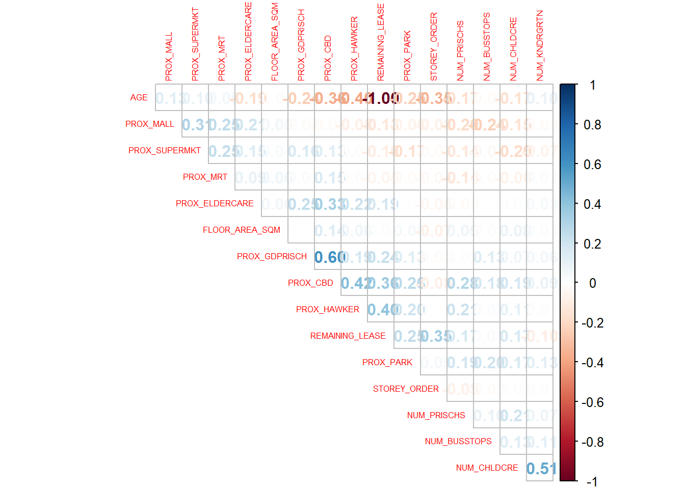
AGE and REMAINING_LEASE are highly correlated (i.e., +/- 0.8):
This makes sense since the older the flat, the lesser the remaining number of years left on the lease.
So we will remove AGEfrom our analysis.
While we did not do this, I found out that one way to improve this part would be to compare AGE amd REMAINING_LEASE to see which variable has a higher correlation to the other variables. We should then remove the one that has a higher correlation to the other variables.
resale_sf <- resale_sf %>% select(-AGE)First we need to split the data into its train and test data sets. We will be using the resale flats in 2022 from June to Decemeber as the train data set and the resale flats in 2023 from January till the end of February as the test data set.
Ideally we should use at least 2 years worth of data for the train data set. Since my laptop is unable to compute such large amounts of data, I have opted to reduce the data set just so I can complete this exercise.
train_sf <- resale_sf %>% filter(month >= "2022-06" & month < "2023-01")
test_sf <- resale_sf %>% filter(month >= "2023-01" & month <= "2023-02")# write them into .rds files for easy access
write_rds(train_sf, "data/model/train_sf.rds")
write_rds(test_sf, "data/model/test_sf.rds")We will be using the lm() function to build the model
# using lm() to get the formula
resale_price.mlr <- lm(formula = resale_price ~ floor_area_sqm + storey_order + remaining_lease +
PROX_CBD + PROX_ELDERCARE + PROX_HAWKER + PROX_MRT + PROX_PARK + PROX_GDPRISCH +
PROX_MALL + PROX_SUPERMKT + NUM_KNDRGRTN + NUM_CHLDCRE + NUM_BUSSTOPS + NUM_PRISCHS,
data = train_sf)
summary(resale_price.mlr)
Call:
lm(formula = resale_price ~ floor_area_sqm + storey_order + remaining_lease +
PROX_CBD + PROX_ELDERCARE + PROX_HAWKER + PROX_MRT + PROX_PARK +
PROX_GDPRISCH + PROX_MALL + PROX_SUPERMKT + NUM_KNDRGRTN +
NUM_CHLDCRE + NUM_BUSSTOPS + NUM_PRISCHS, data = train_sf)
Residuals:
Min 1Q Median 3Q Max
-196561 -26764 -3316 23368 471002
Coefficients:
Estimate Std. Error t value Pr(>|t|)
(Intercept) -1.316e+05 9.849e+03 -13.359 < 2e-16 ***
floor_area_sqm 5.218e+03 1.322e+02 39.466 < 2e-16 ***
storey_order 1.045e+04 4.412e+02 23.682 < 2e-16 ***
remaining_lease 3.897e+03 5.941e+01 65.592 < 2e-16 ***
PROX_CBD -7.615e+00 2.605e-01 -29.236 < 2e-16 ***
PROX_ELDERCARE -3.662e+00 1.505e+00 -2.434 0.0150 *
PROX_HAWKER -6.476e+00 2.073e+00 -3.124 0.0018 **
PROX_MRT -1.564e+01 2.143e+00 -7.297 3.58e-13 ***
PROX_PARK -1.276e+01 2.193e+00 -5.817 6.50e-09 ***
PROX_GDPRISCH -1.473e+00 3.705e-01 -3.975 7.18e-05 ***
PROX_MALL -1.453e+01 2.341e+00 -6.204 6.09e-10 ***
PROX_SUPERMKT 3.076e+01 4.179e+00 7.360 2.24e-13 ***
NUM_KNDRGRTN 6.582e+03 9.963e+02 6.606 4.50e-11 ***
NUM_CHLDCRE -1.921e+03 4.713e+02 -4.076 4.68e-05 ***
NUM_BUSSTOPS 1.296e+03 3.016e+02 4.297 1.78e-05 ***
NUM_PRISCHS -2.656e+03 5.958e+02 -4.457 8.55e-06 ***
---
Signif. codes: 0 '***' 0.001 '**' 0.01 '*' 0.05 '.' 0.1 ' ' 1
Residual standard error: 44990 on 3743 degrees of freedom
Multiple R-squared: 0.7325, Adjusted R-squared: 0.7315
F-statistic: 683.4 on 15 and 3743 DF, p-value: < 2.2e-16With that have the Non-Spatial Multiple Linear Regression Model. Let’s save this into an .rds file so we can always retrieve whenever we want.
write_rds(resale_price.mlr, "data/model/resale_price_mlr.rds")Let’s use the model to predict the resale_price using test data. We will be using the predict() function for this.
train_sf <- read_rds("data/model/train_sf.rds")
test_sf <- read_rds("data/model/test_sf.rds")
resale_price.mlr <- read_rds("data/model/resale_price_mlr.rds")mlr_pred <- predict(resale_price.mlr,
test_sf)
# convert to tbl df
mlr_pred_df <- as.data.frame(mlr_pred)# write it as an rds file to be used later
write_rds(mlr_pred_df, "data/model/mlr_pred_df.rds")Let’s calculate the root mean square error (RMSE) of mlr_pred. This will be used as the main comparison variable with the RMSE of the GWRF model prediction. We will be using the rmse() for this.
# we will need to bind the test data and the mlr_pred to calculate the RMSE
mlr_test_pred <- cbind(test_sf, mlr_pred_df)# write this as an rds file in case we want to access it later
write_rds(mlr_test_pred, "data/model/mlr_test_pred.rds")# calculate the RMSE of the Non-Spatial MLR model
rmse(mlr_test_pred$resale_price,
mlr_test_pred$mlr_pred)[1] 45865.15Please note that the RMSE for the Non-Spatial Multiple Linear Regression Model is 45865.15.
# we will need to use the coordinate data for our GWRF functions
coords_train <- st_coordinates(train_sf)
coords_test <- st_coordinates(test_sf)# write them into rds files
write_rds(coords_train, "data/model/coords_train.rds")
write_rds(coords_test, "data/model/coords_test.rds")We will be using the grf.bw() method for this.
# drop geometry
train_nogeo <- train_sf %>% st_drop_geometry()# write them into rds files
write_rds(train_nogeo, "data/model/train_nogeo.rds")# remember to set seed for simulations
set.seed(1234)
bw_gwrf_adaptive <- grf.bw(formula = resale_price ~ floor_area_sqm +
storey_order + remaining_lease +
PROX_CBD + PROX_ELDERCARE + PROX_HAWKER + PROX_MRT +
PROX_PARK + PROX_GDPRISCH +
PROX_MALL + PROX_SUPERMKT + NUM_KNDRGRTN + NUM_CHLDCRE
+ NUM_BUSSTOPS + NUM_PRISCHS,
train_nogeo,
kernel = "adaptive",
coords = coords_train,
trees = 30)
# write this into rds file
write_rds(bw_gwrf_adaptive, "data/model/bw_gwrf_adaptive.rds")Hm… unfortunately, even after over 30 hours of waiting, the code run did not conclude as the laptop I am currently running this on is not very powerful 😟
Hence, for the purpose of completing this exercise I have no other choice but to estimate the bandwidth for the calibration of the Geographically Weighted Random Forest Model.
When I ran the code, the first bandwidth it tried was 188. At the time of stoppage, the bandwidth it had checked up to was 969. After looking through all the different bandwidths, I found that a bandwidth of 739 yield the highest R2 score of 0.87. Hence I will be using 739 as the bandwidth for my GRF model.
Here is a screenshot of the output from the above code-chunk:
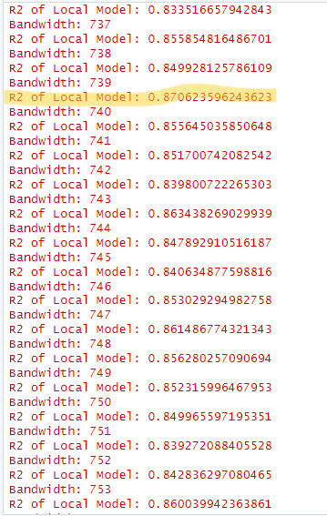
Please note that this is NOT the correct way of building the model and will lead to a much less accurate model. Ideally you should wait for the code chunk to finish running and take the best.bw of the output as the bandwidth to use for the GWRF model calibration.
We will be using the grf() method from the SpatialML package for this. We will be using ntree = 30 for this particular model.
ntree?
The number of trees that the model will grow for each local random forest being generated. We will be making modifications to this argument in Section to see if we can improve the accuracy of the model.
set.seed(1234)
gwrf_adaptive <- grf(formula = resale_price ~ floor_area_sqm +
storey_order + remaining_lease +
PROX_CBD + PROX_ELDERCARE + PROX_HAWKER + PROX_MRT +
PROX_PARK + PROX_GDPRISCH +
PROX_MALL + PROX_SUPERMKT + NUM_KNDRGRTN + NUM_CHLDCRE
+ NUM_BUSSTOPS + NUM_PRISCHS,
dframe=train_nogeo,
bw=739,
kernel="adaptive",
coords=coords_train,
ntree = 30)Ranger result
Call:
ranger(resale_price ~ floor_area_sqm + storey_order + remaining_lease + PROX_CBD + PROX_ELDERCARE + PROX_HAWKER + PROX_MRT + PROX_PARK + PROX_GDPRISCH + PROX_MALL + PROX_SUPERMKT + NUM_KNDRGRTN + NUM_CHLDCRE + NUM_BUSSTOPS + NUM_PRISCHS, data = train_nogeo, num.trees = 30, mtry = 5, importance = "impurity", num.threads = NULL)
Type: Regression
Number of trees: 30
Sample size: 3759
Number of independent variables: 15
Mtry: 5
Target node size: 5
Variable importance mode: impurity
Splitrule: variance
OOB prediction error (MSE): 744755666
R squared (OOB): 0.9011935
floor_area_sqm storey_order remaining_lease PROX_CBD PROX_ELDERCARE
3.559451e+12 3.386695e+12 9.740823e+12 4.518961e+12 4.936195e+11
PROX_HAWKER PROX_MRT PROX_PARK PROX_GDPRISCH PROX_MALL
8.892520e+11 9.166803e+11 5.840046e+11 1.769627e+12 7.871447e+11
PROX_SUPERMKT NUM_KNDRGRTN NUM_CHLDCRE NUM_BUSSTOPS NUM_PRISCHS
3.933218e+11 2.016603e+11 2.411770e+11 1.919996e+11 2.259632e+11
Min. 1st Qu. Median Mean 3rd Qu. Max.
-305000.0 -15010.4 -152.2 -718.5 12429.3 374500.0
Min. 1st Qu. Median Mean 3rd Qu. Max.
-47950.56 -3516.57 -83.33 -0.15 3406.49 50045.56
Min Max Mean StD
floor_area_sqm 16086975278 4.383519e+12 7.656887e+11 1.027084e+12
storey_order 43229925727 3.407597e+12 5.949948e+11 6.456105e+11
remaining_lease 289997155657 7.750744e+12 2.131441e+12 1.903177e+12
PROX_CBD 37918903243 1.635315e+12 3.003264e+11 2.329608e+11
PROX_ELDERCARE 13782170390 5.807095e+11 1.196824e+11 1.152210e+11
PROX_HAWKER 12530717621 1.166765e+12 1.951931e+11 2.130978e+11
PROX_MRT 20366871725 1.155758e+12 2.138980e+11 2.059923e+11
PROX_PARK 22041622500 1.241832e+12 1.783101e+11 1.811973e+11
PROX_GDPRISCH 28910227819 1.082675e+12 2.325057e+11 1.563032e+11
PROX_MALL 16992685964 1.029310e+12 1.368653e+11 1.269357e+11
PROX_SUPERMKT 14429531277 2.977781e+12 1.905317e+11 3.593707e+11
NUM_KNDRGRTN 1492580218 3.553448e+11 3.016804e+10 3.500185e+10
NUM_CHLDCRE 5472959683 2.419665e+11 4.702208e+10 3.224005e+10
NUM_BUSSTOPS 4496659177 3.282395e+11 4.635190e+10 4.338273e+10
NUM_PRISCHS 2696029308 3.940998e+11 4.118088e+10 3.560561e+10# write this into rds file to be used later
write_rds(gwrf_adaptive, "data/model/gwrf_adaptive.rds")We will be using predict.grf() to predict the resale value with the test data and gwrf_adaptive.
local.w and global.w?
These two arguments tell the predict.grf() function how much weight you would like to put on the local model predictor and the global model predictor allowing semi-local predictions.
# combine test data with coordinates data
test_nogeo <- cbind(test_sf, coords_test) %>%
st_drop_geometry()# for now we will be using local.w = 1
gwrf_pred <- predict.grf(gwrf_adaptive,
test_nogeo,
x.var.name = "X",
y.var.name = "Y",
local.w = 1,
global.w = 0)
# convert to tbl df
gwrf_pred_df <- as.data.frame(gwrf_pred)# write this into an rds file to be used later
write_rds(gwrf_pred_df, "data/model/gwrf_pred_df.rds")
write_rds(test_nogeo, "data/model/test_nogeo.rds")# we will need to bind the test data and the mlr_pred to calculate the RMSE
gwrf_test_pred <- cbind(test_nogeo, gwrf_pred_df)
# write this as an rds file in case we want to access it later
write_rds(gwrf_test_pred, "data/model/gwrf_test_pred.rds")
# calculate the RMSE of the Geographically Weighted Regression Model
rmse(gwrf_test_pred$resale_price,
gwrf_test_pred$gwrf_pred)[1] 27312.09Please take note that the RMSE of the Geographically Weighted Model is 27312.09.
As noted in Section 5.5, the MLR model has a RMSE of 45865.15 and the GRF model’s one is 27312.09. This is a huge improvement. We can see that the GRF model has less error than the MLR one. With this we can see that if we want to predict resale prices of HDB flats in Singapore, we need to account for spatial factors. It will be easier to visualise the residuals if we plot the predicted values and the actual resale price onto a scatter plot. So let’s do that.
We will be plotting the residual scatter plots for both the MLR and GRF models for a better comparison between the two.
# plot for GRF
gwrf_plot <- ggplot(data = gwrf_test_pred,
aes(x = gwrf_pred,
y = resale_price)
) + geom_point() + geom_smooth(method=NULL) + ggtitle("GRF Residual Scatter Plot")
# plot for MLR
mlr_plot <- ggplot(data = mlr_test_pred,
aes(x = mlr_pred,
y = resale_price)
) + geom_point() + geom_smooth(method="lm") + ggtitle("MLR Residual Scatter Plot")
# arrange the plots
grid.arrange(mlr_plot, gwrf_plot, ncol = 2)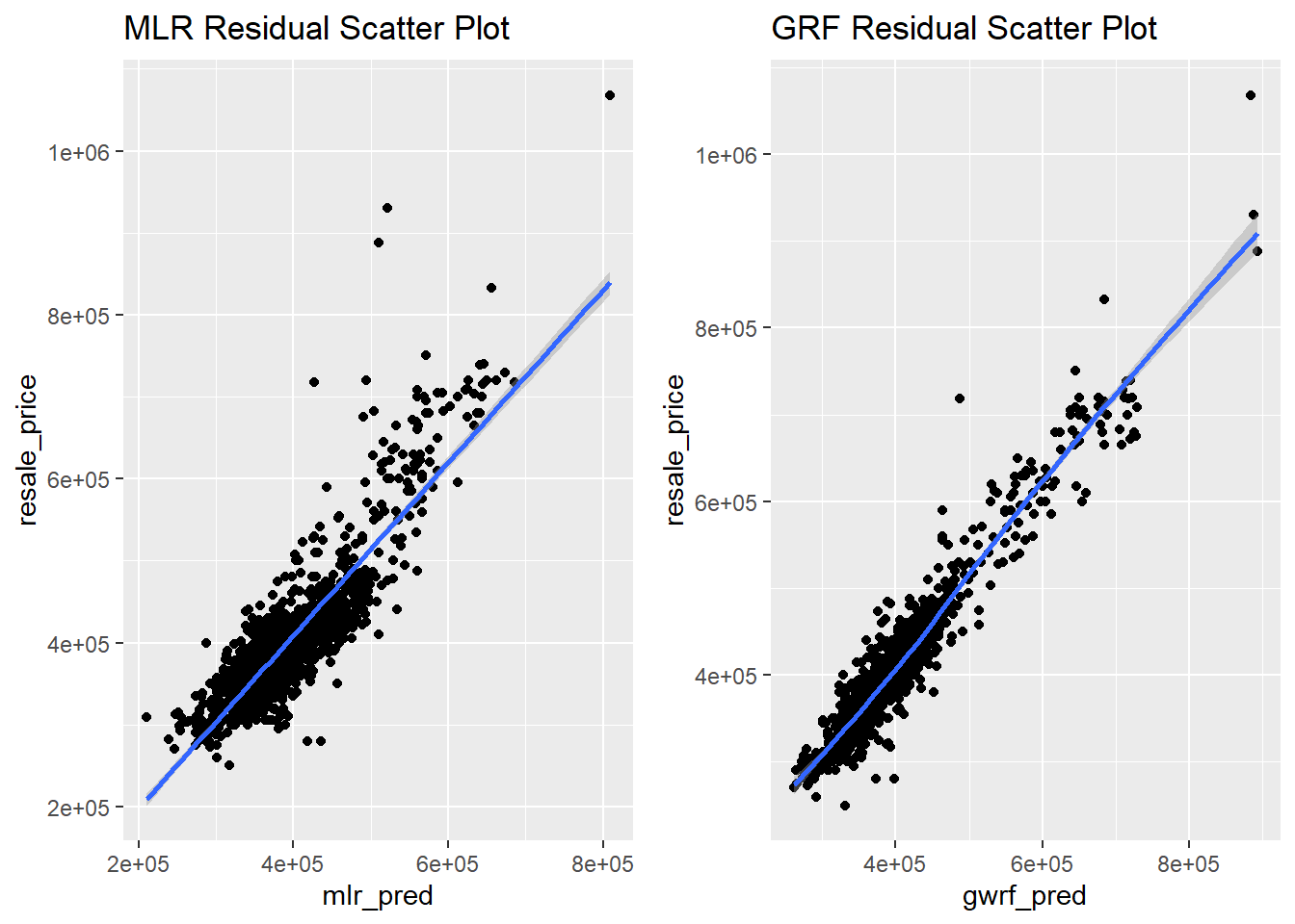
Since the GWRF plot (on the right) has scatter points (i.e., the predicted values) that is closest to the diagonal line (i.e., the actual values), it is the better predictive model.
In this section, we aim to improve the existing GWRF model. I will be attempting to do this by:
ntree argument in the grf() function)local.w and global.w arguments) in the predict.grf() function.My hypothesis is that the predictive performance tends to increase as the number of trees increases. Let’s test to see if this is true.
We will be creating a function that takes in the number of trees and return the RMSE of the prediction model that uses that number of trees. We will then run the function on these options: 30, 40, 50, 60, 70.
all_trees <- list(30,40,50,60,70)ntree_test <- function(tree) {
set.seed(1234)
gwrf_adaptive <- grf(formula = resale_price ~ floor_area_sqm +
storey_order + remaining_lease +
PROX_CBD + PROX_ELDERCARE + PROX_HAWKER + PROX_MRT +
PROX_PARK + PROX_GDPRISCH +
PROX_MALL + PROX_SUPERMKT + NUM_KNDRGRTN + NUM_CHLDCRE
+ NUM_BUSSTOPS + NUM_PRISCHS,
dframe=train_nogeo,
# using the same bw we got from the earlier section
bw=739,
kernel="adaptive",
coords=coords_train,
ntree = tree)
# for now we will be using local.w = 1
gwrf_pred <- predict.grf(gwrf_adaptive,
test_nogeo,
x.var.name = "X",
y.var.name = "Y",
local.w = 1,
global.w = 0)
# convert to tbl df
gwrf_pred_df <- as.data.frame(gwrf_pred)
# we will need to bind the test data and the mlr_pred to calculate the RMSE
gwrf_test_pred <- cbind(test_nogeo, gwrf_pred_df)
# calculate the RMSE of the Geographically Weighted Regression Model
RMSE <- rmse(gwrf_test_pred$resale_price,
gwrf_test_pred$gwrf_pred)
return(RMSE)
}tree_output <- list()
for (tree in all_trees) {
rmse <- ntree_test(tree)
tree_output <- append(tree_output, list(tree = rmse))
}print(tree_output)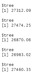
Hm… the results are not what was expected - as the RMSE fluctuates quite a bit. We can conclude that (for this data set and model) using 50 trees gives us a better result than using 30 trees as its RMSE is 26870.06 which is lower than 27312.09.
Now we will be trying to see if we can improve the GWRF model by changing the weight of the local and global model predictors.
local_weights <- list(1, 0.7, 0.3, 0)
global_weights <- list(0, 0.3, 0.7, 1)pred_weight_test <- function(local_w,global_w){
set.seed(1234)
gwrf_adaptive <- grf(formula = resale_price ~ floor_area_sqm +
storey_order + remaining_lease +
PROX_CBD + PROX_ELDERCARE + PROX_HAWKER + PROX_MRT +
PROX_PARK + PROX_GDPRISCH +
PROX_MALL + PROX_SUPERMKT + NUM_KNDRGRTN + NUM_CHLDCRE
+ NUM_BUSSTOPS + NUM_PRISCHS,
dframe=train_nogeo,
# using the same bw we got from the earlier section
bw=739,
kernel="adaptive",
coords=coords_train,
# we will use 50 trees - check previous section
ntree = 50)
# for now we will be using local.w = 1
gwrf_pred <- predict.grf(gwrf_adaptive,
test_nogeo,
x.var.name = "X",
y.var.name = "Y",
local.w = local_w,
global.w = global_w)
# convert to tbl df
gwrf_pred_df <- as.data.frame(gwrf_pred)
# we will need to bind the test data and the mlr_pred to calculate the RMSE
gwrf_test_pred <- cbind(test_nogeo, gwrf_pred_df)
# calculate the RMSE of the Geographically Weighted Regression Model
RMSE <- rmse(gwrf_test_pred$resale_price,
gwrf_test_pred$gwrf_pred)
return(RMSE)
}weight_output <- list()
for (i in 1:length(local_weights)) {
rmse <- pred_weight_test(local_weights[[i]], global_weights[[i]])
weight_output <- append(weight_output, list(weights = rmse))
}print(weight_output)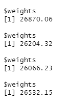
The results show that this model improves as we give a higher weightage to the global model predictor. Hence, we have learnt that for this dataset and model a higher weightage should be given to the global model predictor if we want the lowest RMSE.
Do take note that the RMSE worsens if 0 weightage is given to the local model predictor.